Chapter 36 Practical. Using R
Throughout this book, we have used jamovi for statistical analysis. Jamovi is excellent software for running simple statistical analyses, but it has its limitations. Jamovi is built upon the programming language R, which is much more powerful and versatile in comparison. The R programming langauge is now widely used among scientists for data anslysis. It can be used to analyse and plot data, run computer simulations, or even write slides, papers, or books (this book, including all interactive applications, were written using R). The R programming language is completely free and open source, as is the popular Rstudio software for using it. The R programming language specialises in statistical computing, which is part of the reason for its popularity among scientists.
Another reason for the popularity of R is its versatility, and the ease with which new techniques can be shared. Imagine that you develop a new method for analysing data. If you want other researchers to be able to use your method in their research, then you could write your own software from scratch for them to install and use. But doing this would be very time consuming, and a lot of that time would likely be spent writing the graphical user interface and making sure that your program worked across platforms (e.g., on Windows and Mac). Worse, once written, there would be no easy way to make your program work with other statistical software should you need to integrate different analyses or visualisation tools (e.g., plotting data). To avoid all of this, you could instead just present your new method for data analysis and let other researchers write their own code for implementing it. But not all researchers will have the time or expertise to write their own code.
Instead, R allows researchers to write new tools for data analysis using simple coding scripts. These scripts are organised into R packages, which can be uploaded by authors to the Comprehensive R Archive Network (CRAN), then downloaded by users with a single command in R. This way, there is no need for completely different software to be used for different analyses; all analyses can be written and run in R.
The downside to all of this is that learning R can be a bit daunting at first. Running analyses is not done by pointing and clicking on icons as in jamovi. You need to use code. This practical will start with the very basics and work up to some simple data analyses. Rather than questions to answer, this practical has tasks for you to try to complete in R.
36.1 Getting used to the R interface
There are two ways that you can use R. The first way is to download R and Rstudio on your own computer. Both R and Rstudio are free to download and use, and work on any major operating system (Windows, Mac, and Linux). To download R, go to the Comprehensive R Archive Network and follow the instructions for your operating system (OS). To download Rstudio, go to this page on the Rstudio website and choose the appropriate download for your operating system.
If you cannot or do not want to download R and Rstudio on your own computer, then you can still use both by going to the Rstudio Cloud and running Rstudio from a browser such as Firefox or Chrome. You will need to click the green “Get Started” button and sign up for a free account. When you open Rstudio either on your own computer or the cloud, you will see several windows open, including a console. The console will look something like the below.
R version 4.2.2 Patched (2022-11-10 r83330) -- "Innocent and Trusting"
Copyright (C) 2022 The R Foundation for Statistical Computing
Platform: x86_64-pc-linux-gnu (64-bit)

R is free software and comes with ABSOLUTELY NO WARRANTY.
You are welcome to redistribute it under certain conditions.
Type 'license()' or 'licence()' for distribution details.

  Natural language support but running in an English locale

R is a collaborative project with many contributors.
Type 'contributors()' for more information and
'citation()' on how to cite R or R packages in publications.

Type 'demo()' for some demos, 'help()' for on-line help, or
'help.start()' for an HTML browser interface to help.
Type 'q()' to quit R.

>
If you click to the right of the greater than sign >, you can start using R right in the console.
You can use R as a standard calculator here to get a feel for the console.
Try typing something like the below (semi-colons are not actually necessary).
For example, you could add 2 + 5.
[1] 7Try this yourself.
Task 1: Add 2 numbers together in R
You can also multiply in R.
[1] 16The caret key ^ is used for exponents
[1] 25R will use the correct order of operations (see Chapter 1) when doing mathematical calculations. For example, it will know to calculate the exponent before multiplying, and to multiply before adding.
[1] 102Following the correct order of operations, \(5^{2} = 25\), which is then multiplied by 4 to get \(4 \times 25 = 100\), and we add 2 to get \(100 + 2 = 102\). We can, however, use parentheses to specify a different order of operations.
[1] 150Now R will calculate \(2 + 4 = 6\) and multiply the 6 by 25 to get an answer of 150. The R console functions very well as a calculator. Instead of punching buttons into a hand calculator or mobile phone, an entire equation can be written and placed into the console. This makes mistakes less likely. For example, in Chapter 1.3, the following equation was presented,
\[x = 3^{2} + 2(1 + 3)^{2} - 6 \times 0.\]
To solve this in R, we just need to type the full equation in the console.
[1] 41We get the correct answer of 41.
Note that there needed to be an asterisk (*) to indicate multiplication between the 2 and the left parentheses.
This is because parentheses specify specific functions in R.
We will introduce functions next, but first, try the following task.
Task 2: Use the console to calculate \(x = \frac{2^2 + 1}{3^2 + 2}\) (hint, you need to put the top and bottom of the fraction in parentheses, e.g.,
(2^2 + 1)for the numerator, and use the forward slash/for division).
You should get an answer of 0.4545455.
As previously mentioned, parentheses specify functions in R.
Functions have specific names such as sqrt, which calculates the square root of anything within the parentheses sqrt().
If, for example, you wanted to find the square root of some number, you could use the sqrt function below.
[1] 16The console returns the correct answer 16.
Similar functions exist for logarithms (log) and trigonometric functions (e.g., sin, cos).
The parentheses after the word indicate that some function is being called in R.
Try to use the square root function to solve for \(x\) in another equation.
Task 3: Use the console to calculate \(\sqrt{3 + 4^2}\).
You should get an answer of 4.3588989.
If you type something into the console incorrectly, you do not need to retype it entirely. You can use the up arrow to scroll through the history of console input. Try doing that now.
Task 4: Use the up arrow to find your previous calculation for \(\sqrt{3 + 4^2}\), then change this slightly to calculate \(\sqrt{3 + 4^3}\).
You should get an answer of 8.1853528.
Functions do not need to be mathematical like the sqrt function.
For example, the getwd function can be used to let you know what directory (i.e., folder) you are working in.
[1] "/home/brad/Dropbox/teaching/modules/SCIU4T4/statistical_techniques"If we were to save or load a file within R, this is the location on the computer from which R would try to load.
We could also use the setwd function to set a new working directory (type the working directory in quotes inside the parentheses: setwd("folder/subfolder/etc")).
You can also set the working directory in Rstudio by going to the toolbar and clicking ‘Session’ and selecting ‘Set Working Directory’.
36.2 Assigning variables in the R console
In R, we can also assign values to variables using the characters <- to make an arrow.
For example, we might want to set var_1 equal 10.
We can now use var_1 in the console.
For example, since var_1 now equals 10, if we multiply var_1 by 5, R calculates \(10 \times 5 = 50\).
[1] 50The correct value of 50 is returned because var_1 equals 10. Also note the comment left after the # key.
In R, anything that comes after # on a line is a comment that R ignores.
Comments are ways of explaining in plain words what the code is doing, or drawing attention to important notes about the code.
Task 5: Assign a new variable to a value of 4 (call it anything you want), then multiply the new variable by itself.
For Task 5, you should get an output of 16.
When we assign something to a variable like var_1, we are not limited to a single number.
Variables in R can be much more complex.
For example, we can assign a new variable vector_1 to an ordered set of 6 different numbers using the c function.
The c function combines values together.
[1] 5 1 3 5 7 11Doing this makes it possible to calculate for all of the values in vector_1 at the same time.
We might, for example, want to multiply all of the numbers by 10.
[1] 50 10 30 50 70 110Variables also do not necessarily need to be numbers.
We might assign a new variable phrase_1 to a string of letters.
When doing this, the letters need to be enclosed in quotation marks.
[1] "string of words"We can even combine numbers, vectors, and words into a single object as a list using the list function.
[[1]]
[1] 10

[[2]]
[1]  5  1  3  5  7 11

[[3]]
[1] "string of words"
There are far too many possibilities to introduce everything about how R works. The best way to get started is to play around and see what works and what does not. You will not break anything. Error messages are good because they can help you learn how R works.
Task 6: Use the R console until you find a new error message.
Try something new in the R console. Keep going until you get an error message that you have not yet seen, then move on to the next exercise.
36.3 Some descriptive statistics
Now we can get started with some statistical analyses.
In Chapter 38 we will learn how to do some familiar analyses with R scripts and data uploaded from CSV files, but for now, we will just type our data directly into the console.
We can use the data from Chapter 35 as an example.
The code below reads in 2 different variables, SO1 and SO2.
The numbers are the same ovipositor lengths from the histograms in Figure 35.2 of Chapter 35.
SO1 <- c(3.256, 3.133, 3.071, 2.299, 2.995, 2.929, 3.291, 2.658, 3.406,
         2.976, 2.817, 3.133, 3.000, 3.027, 3.178, 3.133, 3.210);
SO2 <- c(3.014, 2.790, 2.985, 2.911, 2.914, 2.724, 2.967, 2.745, 2.973,
         2.560, 2.837, 2.883, 2.668, 3.063, 2.639);
Copy and paste the code above into the R console.
You should now have 2 new variables, SO1 and SO2
Task 7: Type
SO1into the R console to print the ovipositor lengths for species SO1, then do the same forSO2.
We can replicate the histogram from Figure 35.2A in Chapter 35 with the following code.
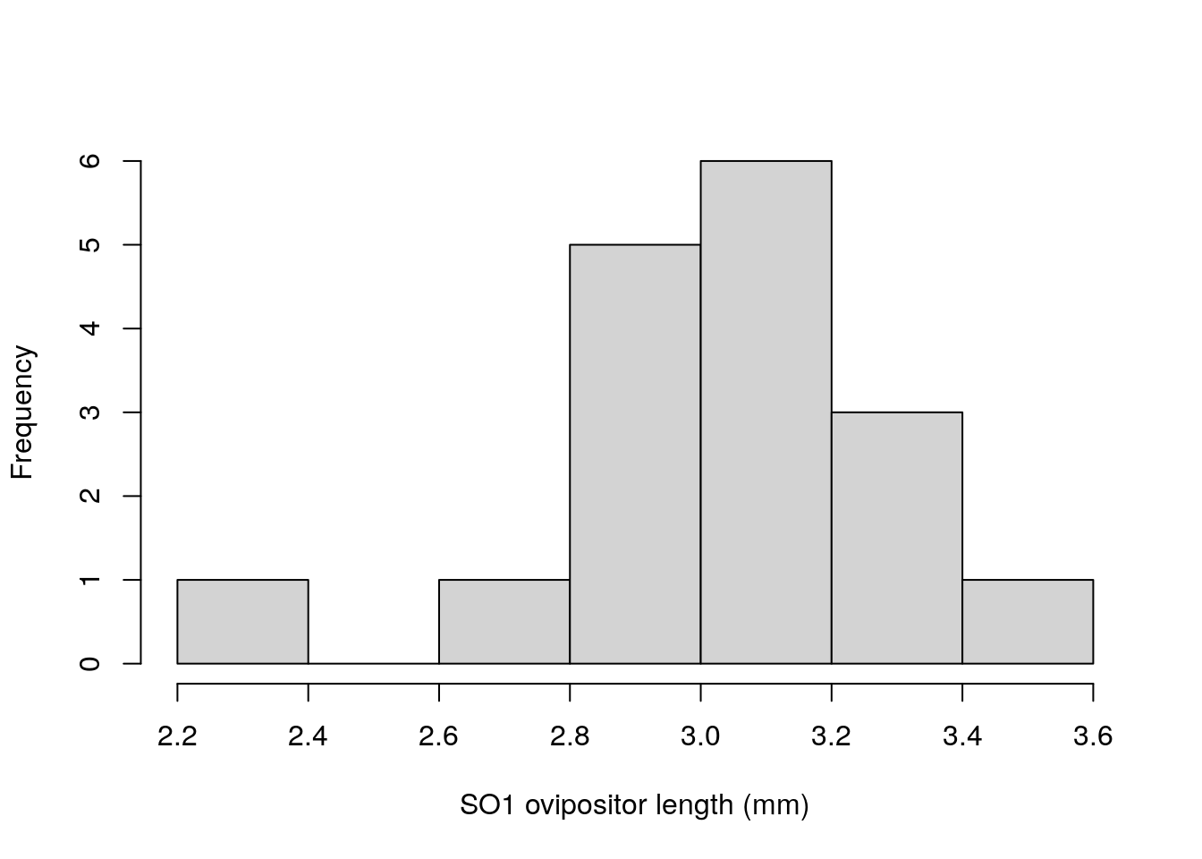
Figure 36.1: Ovipositor length distributions for an unnamed species of fig wasps SO1.
The bin widths in Figure 36.1 are not the same as Figure 35.2A because there are other options within hist that have not been specified.
Within hist and other functions, these options such as x, xlab, and main are called arguments.
The word ‘argument’ in this case has nothing to do with a disagreement or logical reasoning.
In this case, it just refers to information that is passed in a function.
Task 8: Make a histogram of SO2 ovipositor lengths. Try using the argument
col = "blue"in thehistfunction to make the histogram bars blue.
Now we can try collecting some summary statistics for SO1 and SO2. In the lab practical from Chapter 14, we used jamovi to calculate summary statistics. Table 36.1 below shows how those same summary statistics can be calculated using functions in R, and the output of each function for SO1.
| Statistic | Function | Output |
|---|---|---|
| N | length(SO1) |
17 |
| Std. deviation | sd(SO1) |
0.260018 |
| Variance | var(SO1) |
0.067609 |
| Minimum | min(SO1) |
2.299 |
| Maximum | max(SO1) |
3.406 |
| Range | range(SO1) |
2.299, 3.406 |
| IQR | IQR(SO1) |
0.202 |
| Mean | mean(SO1) |
3.030118 |
| Median | median(SO1) |
3.071 |
Notice that the range function gives the minimum and maximum of SO1, so we need to subtract the latter from the former to get the actual range.
Task 9: Calculate the summary statistics in Table 36.1 for SO2.
There is no function for standard error in R. We could write a custom function to calculate the standard error, but for now we can just use the formula from Chapter 12 to calculate the standard error of SO1,
\[SE = \frac{s}{\sqrt{N}}.\]
Since we have the standard deviation (\(s\)) and sample size (\(N\)) from Table 36.1, we can calculate SE in R,
[1] 0.06306363The code above calculates the standard deviation of SO1 (sd(SO1)), then divides (/) by the square root (sqrt()) of the length of SO1 (length(SO1)).
This can be difficult to read because length(SO1) is enclosed in sqrt().
But we can break this down step by step to make it easier to read by assigning each component to a new variable.
SO1_SD <- sd(SO1);     # Assign the standard deviation
SO1_N  <- length(SO1); # Assign the N
SO1_SD / sqrt(SO1_N);  # Do the calculation for SE
[1] 0.06306363We can do the same for SO2.
Task 10: Calculate the standard error of SO2 ovipositor lengths.
With the standard error now calculated, we can also calculate 95 per cent confidence intervals using the formula from Chapter 18, just as we did for SO1 in Chapter 35,
\[LCI = 3.03 - \left(2.120 \times \frac{0.26}{\sqrt{17}}\right),\]
\[UCI = 3.03 + \left(2.120 \times \frac{0.26}{\sqrt{17}}\right).\]
Note that 3.03 is the mean from Table 36.1, and \(0.26/\sqrt{17}\) is the standard error that we just calculated for SO1. The value 2.120 is the t-score associated with df = 17 - 1, i.e., 16 degrees of freedom (see Chapter 35). As in Chapter 35, we get values of LCI = 2.896 and UCI = 3.164.
Task 10: Calculate 95 per cent confidence intervals for SO2 ovipositor lengths (hint: the appropriate t value for df = 14 is 2.145 instead of 2.120).
In the last exercise, we will attempt to bootstrap these confidence intervals using the method introduced in Chapter 35.
36.4 Bootstrapping confidence intervals
Writing resampling and randomisation procedures in R requires some knowledge of coding.
For now, all that you need to do is copy a pre-defined function into R and use it like any other function.
The function is called simpleboot.
simpleboot <- function(x, replicates = 1000, CIs = 0.95){
  alpha <- 1 - CIs;
    vals  <- NULL;
    i     <- 0;
    while(i < replicates){
        boot  <- sample(x = x, size = length(x), replace = TRUE);
        strap <- mean(boot);
        vals  <- c(vals, strap);
        i     <- i + 1;
    }
    vals   <- sort(x = vals, decreasing = FALSE);
    lowCI  <- vals[round((alpha*0.5)*replicates)];
    highCI <- vals[round((1-(alpha*0.5))*replicates)];
    confid <- c(lowCI, highCI);
    return(list(vals, confid));
}
The simpleboot function takes a variable (x) as an argument, bootstraps mean values replicates times, and produces confidence intervals at a level CIs.
To use it, highlight and copy the entire function, then put it into the R console.
Make sure that every line from simpleboot to the last } is copied.
Once it has been placed into the R console, it can be used just like any other function.
For example, we can run simpleboot and store the output for SO1 values.
The output will include a list of 2 different objects.
The first object SO1_95s[[1]] will be a list of 1000 bootstrapped mean values, sorted from lowest to highest.
The second object SO1_95s[[2]] will be the bootstrapped upper and lower confidence intervals.
First, we can take a look at a histogram of the bootstrapped mean values.
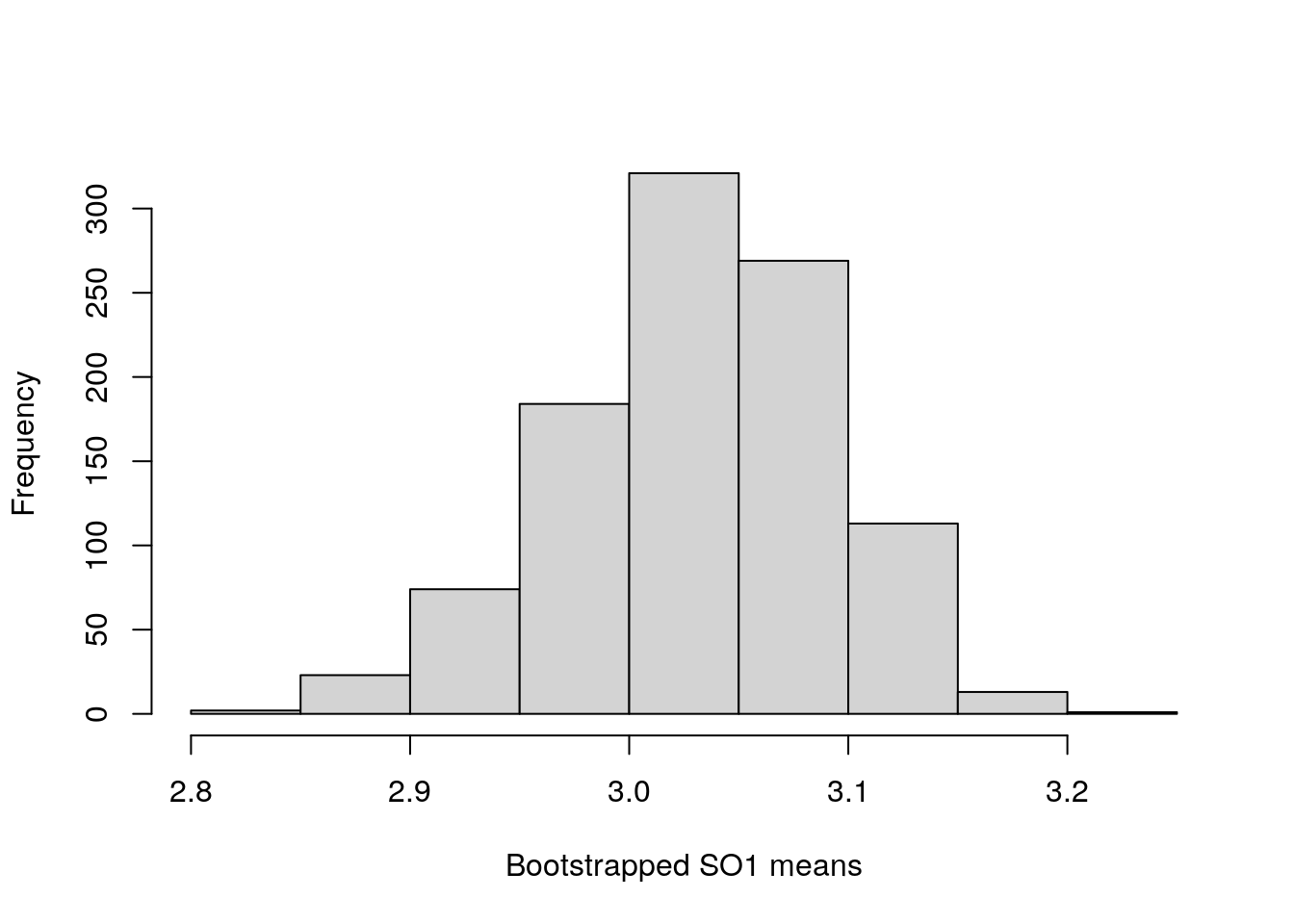
Figure 36.2: Bootstrapped mean values for 17 ovipositor lengths in an unnamed species of fig wasp collected in Baja, Mexico.
We can then print out the lower and upper confidence intervals, which report the value of the 2.5 per cent rank and 97.5 rank bootstrapped means, respectively.
[1] 2.902059 3.146706Note that these values are not too far off the values of LCI = 2.896 and UCI = 3.164 calculated in the usual way in the previous exercise.
Task 11: Use the
simplebootfunction to calculate 95 per cent confidence intervals for SO2 mean ovipositor lengths.
The practical in Chapter 38 will demonstrate how to read CSV files into R and run hypothesis tests, including t-tests, ANOVAs, chi-square tests, correlation tests, and linear regression.