Chapter 38 Practical. Statistical techniques in R

This lab practical will demonstrate how to run statistical tests in R that have been introduced in jamovi in previous practicals. The practical will use the PalmerPenguins dataset (Gorman, Williams, and Fraser 2014; Horst, Hill, and Gorman 2020). These data include morphological measurements for 3 species of penguins that inhabit 3 islands in the Palmer Archipelago, Antarctica (Figure 38.1; artwork by allison_horst, Creative Commons Attribution 4.0 International License).

Figure 38.1: This practical uses data collected on the morphologies of 3 Antarctic penguin species.

The data were collected by Dr Kristen Gorman at the Palmer Station Long Term Ecological Research program from 2007-2009. To complete this lab, download the penguins.csv dataset (right click and “Save Link As…”, then save it with the extension ‘.csv’). Data include measurements of bill length (mm), bill depth (mm), flipper length (mm), body mass (g), and sampling year for penguins of 3 species on 3 islands.

38.1 Working with a data set

First, we need to open Rstudio. You can do this on your own computer, or within a browser on the posit cloud. Although it is possible to use R in a different environment than Rstudio, Rstudio will make some tasks easier. To get started, we need to make that we are working in the same directory (i.e., folder, see Chapter 2 on managing data files) that we saved the penguins.csv. We could use the setwd() function to do this (e.g., by typing something like setwd("C:\Users\MyName\Documents") in the console on a Windows computer). But the easiest way in Rstudio is to navigate to the toolbar and select ‘Session’, then ‘Set Working Directory’ from the pulldown, and then ‘Choose Directory’ (Figure 38.2).

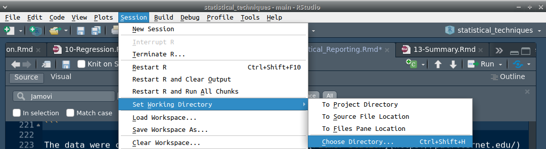
Figure 38.2: Rstudio option in the toolbar for setting a working directory.

A new window will open that will allow you to navigate to the location in which penguins.csv was saved.

In the practical from Chapter 36, we worked entirely from the R console. This time, we will will introduce R scripts to make organising the code a bit easier. To do this, navigate to the Rstudio toolbar and select ‘File’, then ‘New File’ followed by ‘R Script’ (Figure 38.3).

Figure 38.3: Rstudio option in the toolbar for creating a new R script.

You should then see an empty script called ‘Untitled1’ open up above the R console. This will be useful because it will allow us to save the R commands that we run.

Task 1: Open a new R script by selecting ‘File > New File > R script’.

Now we need to read in the penguins dataset. Assuming that we are in the same working directory as the place we saved the file called ‘penguins.csv’, we can use the function read.csv to read in the CSV file. Type (or copy-paste) the line below into the R script.

penguins <- read.csv(file = "penguins.csv");

Put your cursor on the line that you typed (you can also highlight the whole line, but this is not necessary). Next, find the ‘Run’ button in the toolbar and click it (Figure 38.4). Rstudio will run whatever line of code your cursor is on, or whatever chunk of code is highlighted (including multiple lines at once; notice the line numbers in the left margin of the script).

Figure 38.4: An Rstudio toolbar with the ‘Run’ option in the upper right to run a line of code from the script to the console.

If that did not work, then double-check to make sure that you are in the correct directory and have the file name correct. Everything in R is case sensitive, meaning that capitalisation matters, so R will treat ‘Penguins.csv’ and ‘penguins.csv’ as completely different! It is important to be precise.

Once you have read in the penguins dataset, have a look at the first 6 rows using the function head.

Task 2: View the first 6 rows of the penguins dataset.

On the second line of your R script, type the code below, then run it.

head(penguins);

  species    island bill_length bill_depth flipper_length mass  year
1  Adelie Torgersen        39.1       18.7            181 3750 Y2007
2  Adelie Torgersen        39.5       17.4            186 3800 Y2007
3  Adelie Torgersen        40.3       18.0            195 3250 Y2007
4  Adelie Torgersen          NA         NA             NA   NA Y2007
5  Adelie Torgersen        36.7       19.3            193 3450 Y2007
6  Adelie Torgersen        39.3       20.6            190 3650 Y2007

You should see the first 6 rows of the dataset print out in the console. Notice that the dataset is already in a tidy format. Each row is an individual penguin, and each variable is a column.

Unlike jamovi, we cannot change the data in penguins simply by clicking on values. Like everything else in R, we need to do this using code. If we wanted to change the value of row one column three to 40, for example (i.e., the first penguin’s bill depth), then we would need to do the following.

penguins[1, 3] <- 40

The square brackets can be used to indicate a specific row and column in the data (i.e., data[row_number, column_number]). A missing value in the square brackets will be interpreted by R as referring to all elements in the dataset. For example, if we wanted to have R just print off the fifth row of the penguins dataset, we could run the following.

penguins[5, ]

The absence of any value above in , ] tells R to print all of the columns. We can do the same for the columns.

Task 3: Print just column 3 of the penguins dataset. What does the code look like?

Code to return column 3: ______________

Notice that some of the values in the dataset are not numeric, but instead are given as NA. This is how missing data are indicated in R. An example of this is shown in the measurements for the penguin in the fourth row. These NA values can become a nuisance when we try to calculate summary statistics. Using the mean function introduced in the practical last week, try running the line of code below to get the mean of column 3.

mean(x = penguins[,3])

We get a value of NA instead of the mean of the numbers that are not missing. This is because we need to tell R explicitly to remove values that are missing when calculating the mean. We can do this with the na.rm argument in the mean function.

mean(x = penguins[,3], na.rm = TRUE)

Note that we can also access column three by using the $ sign and the name of the relevant column (in this case bill_length). We could therefore get the same answer as above using the code below.

mean(x = penguins$bill_length, na.rm = TRUE)

There is usually more than one way of doing the same thing in R (we could also use penguins[["bill_length"]]).

Task 4: Find the mean bill length of penguins in mm (column 3)

Mean bill length (mm): ____________________

Now we can try 2 more functions. The function sd returns the standard deviation of numbers (note that while na.rm is not an argument for every R function, it can also be used as an argument in sd). The function length returns the length of an object. Try using these functions to calculate the 95 per cent confidence intervals for mean bill length (you can use a z-score of 1.96).

Task 5: Calculate lower and upper confidence intervals (CIs) using the R functions mean, sd, and length.

Lower bill length CI: ______________________

Upper bill length CI: ______________________

Next, we can use the penguins dataset to run a one-way ANOVA, two-way ANOVA, \(\chi^{2}\) tests, correlation test, and linear regression. This practical will walk you through the code so that you can focus on understanding the R output.

38.2 Familiar statistical tests in R

In this exercise, we will use the penguins dataset to run some familiar statistical hypothesis tests. In R, there is typically more than one way to do something. We will focus on the simplest way to run a one-way ANOVA, two-way ANOVA, \(\chi^{2}\) tests, correlation test, and linear regression.

38.2.1 One-way ANOVA in R

We can start by running a one-way ANOVA to test the null hypothesis that all species have the same mean bill length. Normally we would want to first check the assumptions of the ANOVA. For now, we will assume that no assumptions are violated, but the Shapiro-Wilk test and Levene’s test of equal variances will be demonstrated later. To run a one-way ANOVA in R, we can use the code below.

anova_model <- lm(formula = bill_length ~ species, data = penguins);
anova(anova_model);

The function lm runs a general linear model (we have not discussed it in this module, but t-tests, ANOVA, and linear regression are all based on the same mathematical framework; see Chapter 39 for more explanation). We can use the column names bill_length and species directly if we specify that we are using the dataset in which these columns are found (penguins). Inside lm, you will notice the ~ symbol. This just separates our dependent variable (bill_length on the left) and independent variable (species on the right).

In the above, we are storing this model with a new variable named anova_model (note that we can use <- to store more than just lists of numbers; in this case, our object is the whole linear model!). The function anova then summarises this model.

Task 6: Use the code above to run an ANOVA to test the null hypothesis that species have the same bill length. Find the F value and p value from the output.

Note that R uses scientific notation to write very low values. For example 5.5e-4 would be interpreted as \(5.5 \times 10^{-4}\), which is 0.00055.

F value: _________________

p value: _________________

Since our p-value is less than 0.05, we can also run a Tukey’s Honestly Significant Difference test of multiple comparisons (see Chapter 25). We need to use the aov and TukeyHSD functions to do it.

TukeyHSD(aov(anova_model));

The TukeyHSD function will report a table of post hoc comparisons similar to the ones reported by jamovi.

38.2.2 Two-way ANOVA in R

We can run a two-way ANOVA using the independent variables ‘species’ and ‘year’ with the code below.

two_way_aov <- lm(formula =  bill_length ~ species + year + species:year, 
                  data = penguins);
anova(two_way_aov);

Note that the code above looks very similar to our one way ANOVA. Now we are just adding a new independent variable with the + sign, and adding an interaction between species and island, which is written as species:year.

Task 7: Use the code above to run a two way ANOVA. Determine whether or not the the main effects of the model (species and year) are significant, and whether the interaction terms are significant.

Significance:

Species? __________

Year? _____________

Interaction? _____________

38.2.3 Chi-square test in R

To run a \(\chi^{2}\) goodness of fit test, we need to first put the data in a table form. Suppose that we wanted to test the null hypothesis that penguins were sampled from equal frequencies across all islands. We can use the table function in R to first build a contingency table of counts of penguins observed on each island.

island_table <- table(penguins$island);
print(island_table);

   Biscoe     Dream Torgersen 
      168       124        52 

The contingency table generated using the table function reveals that there were 168 penguins observed on the island Biscoe, 124 penguins observed on the island Dream, and 52 penguins observed on the island Torgersen. To run a \(\chi^{2}\) goodness of fit test, we can use the island_table that we just created in the function chisq.test.

chisq.test(island_table);

The output of chisq.test will include the \(\chi^{2}\) statistic (‘X-squared’), the degrees of freedom (‘df’), and the p-value.

Task 8: Use the code above to run a Chi-square goodness of fit test. Report the test statistic below.

\(\chi^{2}\) test statistic: _____________________

A \(\chi^{2}\) test of association also requires counts to be placed in the format of a contingency table. This can be done by including 2 variables as arguments in table. We can build a contingency table of penguin counts for each island.

sp_island_table <- table(penguins$island, penguins$species);
print(sp_island_table);

           
            Adelie Chinstrap Gentoo
  Biscoe        44         0    124
  Dream         56        68      0
  Torgersen     52         0      0

The chisq.test function can then be run directly with this new table sp_island_table as an argument to run a \(\chi^{2}\) test of association.

chisq.test(sp_island_table);

Task 9: Use the code above to run a Chi-square test of association between penguin species and island counts. Report the test statistic below.

\(\chi^{2}\) test statistic: _____________________

38.2.4 Correlation test in R

We can now look at how to find the correlation between two variables in R, and how to test whether or not they are significant. Suppose that we want to test whether or not bill length and flipper length are correlated in penguins. We can do this with the cor.test function in R.

cor.test(x = penguins$bill_length, y = penguins$flipper_length, 
         alternative = "two.sided", method = "pearson");

Notice that the cor.test function makes it possible to specify the alternative hypothesis (“two.sided”, “less”, and “greater”). It also is possible to use a Spearman correlation coefficient (method = “spearman”) instead of a Pearson product moment correlation coefficient.

Task 10: Run a test of the null hypothesis that the Pearson correlation coefficient between bill length and flipper length is zero. Report the correlation coefficient r below.

r: _________________

Note that the output of the correlation test includes the t statistic, which is used for correlation hypothesis testing (Chapter 30). It also includes 95 per cent confidence itnervals around \(r\), degrees of freedom, and the p-value (note that 2.2e-16 just means \(2.2 \times 10^{-16}\), i.e., a very small number).

38.2.5 Simple linear regression in R

Suppose we want to try to predict penguin body mass from bill length. How would we run a simple linear regression for this in R? The code is actually very similar to what we used for running an ANOVA. We can again use the function lm. For simplicity, and because the goal here is just to show how to use the R functions, we will just assume that all of the relevant assumptions of regression are true. In this case, our linear model can be run using the code below.

lin_mod <- lm(formula = mass ~ bill_length, data = penguins);
summary(lin_mod);

In the above code, the first line defines the model (lin_mod), and the second line summarises it for us with the output we need to make conclusions. Notice that the first line has the exact same structure as we used in the ANOVA. In the formula, the dependent variable mass is separated from the independent variable bill_length with the ~ character, and we specify the dataset for both variables (penguins).

Task 11: Examine the output of the simple regression of penguin body mass against bill depth from the code above. Find the R-squared value (called ‘Multiple R-squared’), intercept, slope, and p-value for the overall model.

R-squared: _______________

Intercept: _______________

Slope: ___________________

Model p-value: ___________

Note that the p-value for the model is in the very bottom right of the output.

38.2.6 Multiple regression in R

Now we can add to the complexity of our model by including another independent variable. Suppose we want to predict body mass from both bill length and flipper length. Again, assume that all of the assumptions of regression are met; the goal is just to show the R functions at work. For multiple regression, the code again looks suspiciously similar to what it does for a two-way ANOVA (note, we should really also consider an interaction between our independent variables in multiple regression too, but for now we will just assume that none exists).

mult_regr <- lm(formula = mass ~ bill_length + bill_depth, 
                data = penguins);
summary(mult_regr);

The output above looks similar to that of our simple linear model, but we now have a coefficient and p-value for an additional independent variable (bill depth).

Task 12: Examine the output of the multiple regression from the code above. Find the adjusted R-squared value, and write down the equation of the model.

Adjusted R-squared: ________________

Model equation: ____________________

We have now looked at how to run ANOVAs, Chi-square tests, correlation tests, and regression in R. These tests rely on assumptions about the data. If these assumptions are violated, then we need to run a nonparametric alternative test. The next section will demonstrate how to test whether or not data are normally distributed and if groups have equal variances.

38.3 Statistical test assumptions in R

In the one-way ANOVA of Chapter 38, we tested if bill length differed among penguin species. An assumption of the ANOVA is that the data are normally distributed and groups have equal variances. We can run a Shapiro-Wilk test to check if data are normally distributed using the shapiro.test function in R.

shapiro.test(x = penguins$bill_length);

Task 13: Test if penguin bill length is normally distributed.

Based on this test, is bill length normally distributed? __________

We can also check to see if species bill lengths have equal variances. We can do this using a Levene’s test of homogeneity of variances, as we have done in jamovi. The base functions of the R programming language do not include a Levene’s test. We therefore need to download an R package that has a function for the Levene’s test. Packages in R include code that people have written and made available to other researchers. The Comprehensive R Archive Network (CRAN) includes thousands of R packages that can be used to run all kinds of different functions. The package that we need is called ‘car’, and we can download it from CRAN using the install.packages function.

install.packages("car");
library("car");

The install.packages("car") installs the ‘car’ package, and the library("car") loads it into R so that the functions in the package can be used. One of these functions is called leveneTest, which we can use to run the Levene’s test of homogeneity of variances.

leveneTest(bill_length ~ species, data = penguins);

Task 14: Use the ‘car’ R package to run a Levene’s test, then report the p-value of the test below.

P: __________________

Remember that the Levene’s test tests the null hypothesis that group variances are the same. Hence, if \(P > 0.05\), we should not reject the null hypothesis of equal variances. Nevertheless, from the earlier Shapiro-Wilk test, it appears that the data are not normally distributed. Instead of using a one-way ANOVA, we should therefore try the non-parameteric equivalent Kruskall-Wallis H test (Chapter 26). The Kruskall-Wallis H test can be run in R using the kruskal.test function.

kruskal.test(bill_length ~ species, data = penguins);

Recall from Chapter 26 that the Kruskall-Wallis H test uses a \(\chi^{2}\) test statistic.

Task 15: Run a Kruskall Wallis H test to see if bill length differs among species, then report the \(\chi^{2}\) test statistic of the test below.

\(\chi^{2}\): ___________________

There is much, much more that we could do in R. But once you understand the general idea of how R works, the best thing to do is play around with R code. If you want to run a specific statistical test, then it is almost certain that the test can be run in R. You might just need to search for the relevant function or R package online.

References

Gorman, Kristen B, Tony D Williams, and William R Fraser. 2014. “Ecological Sexual Dimorphism and Environmental Variability Within a Community of Antarctic Penguins (Genus Pygoscelis).” PloS One 9 (3): e90081.

Horst, Allison Marie, Alison Presmanes Hill, and Kristen B Gorman. 2020. Palmerpenguins: Palmer Archipelago (Antarctica) Penguin Data. https://doi.org/10.5281/zenodo.3960218.