Advanced techniques
A Bradley Duthie
2025-05-01
Source:vignettes/advanced_techniques.Rmd
advanced_techniques.RmdIntroduction
Here we focus on advanced techniques for simulating pest ecological and evolutionary dynamics using the resevol R package. In the main text, we provided a simple example of individual-based simulations to demonstrate how to get started. This document focuses instead on demonstrating the more advanced options of the package and showcasing what it can do. The case study will focus on crop and pesticide rotation on a complex, customised landscape that includes farmland, grassland, forest, and water. The pest species will be sexually reproducing and obligately biparental, and its life history will include an egg and larval stage during which it feeds on crops and consumes pesticide, and a stage during which it moves, mates, and reproduces. The pest species will include a total of four evolving traits that affect the consumption of two crops and two pesticides. The objective of simulations will be to test how pest population size changes and traits evolve given different pesticide rotation regimes. Below, we explain how to model this system in detail, including all of the necessary code for reproducing the example within the text.
Initialising pest genomes
First, we need to use the mine_gmatrix function to
initialise pest genomes. In our example, individuals will have four
covarying traits resulting from 12 loci. There will be 4 internal nodes
that map loci values to traits (see the Evolutionary Algorithm
explanation for details). The trait covariance structure will be defined
as below.
library("resevol");
gmt <- matrix(data = c(1.0, -0.5, 0.2, 0.2, -0.5, 1.0, 0.2, 0.2, 0.2,
                       0.2, 0.4, -0.6, 0.2, 0.2, -0.6, 0.4), nrow = 4);
print(gmt);
## [,1] [,2] [,3] [,4]
## [1,] 1.0 -0.5 0.2 0.2
## [2,] -0.5 1.0 0.2 0.2
## [3,] 0.2 0.2 0.4 -0.6
## [4,] 0.2 0.2 -0.6 0.4Rows and columns 1 and 2 will represent traits underlying the
consumption rate of crops 1 and 2, respectively. Hence, the variation in
crop consumption rate is 1 for both crops, while the covariance in
consumption rate is -0.5, meaning that there is a trade-off between pest
ability to consume crop 1 versus crop 2. Rows and columns 3 and 4 will
represent traits underlying the consumption rate of pesticides 1 and 2,
respectively. Hence, the variation in pesticide consumption rate is 0.4
for both pesticides, which is lower than what it is for crops. There is
a trade-off in the consumption rate of pesticide 1 versus pesticide 2,
which is reflected in the covariance of -0.6 in the above matrix.
Finally, there is a positive covariance of 0.2 between all crop and all
pesticide consumption rates. What this means is that pests that consume
crops quickly also tend to consume pesticides quickly, causing a
potential trade-off between the beneficial effects of feeding ability
and the negative effects of pesticides. We can now use the
mine_gmatrix function to find a network mapping loci to
traits that satisfies the above trait covariance structure. The options
used below in mine_gmatrix arguments will lead to a
computationally intense (and therefore time-consuming) search,
particularly due to the large number of networks in the population
(npsize = 12000), high number of individuals used to test
network stress (indivs = 2000), high number of hidden nodes
(layers = 4), strict stress criteria
(term_cri = -8), and high maximum generation number
(max_gen = 5400).
set.seed(2022);
mg  <- mine_gmatrix(gmatrix = gmt, loci = 12, indivs = 2000, npsize = 12000,
                    max_gen = 5400, sampleK = 1200, chooseK = 6, layers = 4,
                    mu_pr = 0.2, pr_cross = 0.2, mu_sd = 0.004,
                    term_cri = -8);
To save time, a genome mg produced from the code above
has been saved into the resevol R package as
advanced_techniques_eg.rda, which we can load. Note that
running mine_gmatrix can be a time-consuming process, and
will often require multiple attempts to get the above parameter settings
to produce a desired network. See Hamblin (2013) for useful advice on parameter
value selection for the evolutionary algorithm. Time-sensitive parameter
values specific to the resevol package include indivs and
layers. Increasing values for both of these parameters can
increase run time.
load(system.file("advanced_eg.rda", package = "resevol"));The contents of each list element of mg are not
important for our purposes, but an explanation is available in the package documentation. What is
important is the sixth list element, which holds the estimated
covariance structure found by the evolutionary algorithm.
##            [,1]       [,2]       [,3]       [,4]
## [1,]  1.0677123 -0.4510309  0.1225596  0.1277905
## [2,] -0.4510309  1.0449414  0.1251180  0.1217368
## [3,]  0.1225596  0.1251180  0.5014936 -0.3992066
## [4,]  0.1277905  0.1217368 -0.3992066  0.5011398
We can compare the above covariance structure with the one that we
specified in gmt. The stress of mg (i.e., mean
squared deviation of mg elements from gmt
elements) is 0.0099034. But this is only based on one population of
indivs = 2000 initialised pests. We can use the
stress_test function to see what the distribution of stress
is over 1000 such initialised populations of 2000 individuals (Figure
1).
sim_stress <- stress_test(mine_output = mg, indivs = 2000, reps = 1000);
hist(x = sim_stress, main = "", breaks = 20, xlab = "Initialised stress");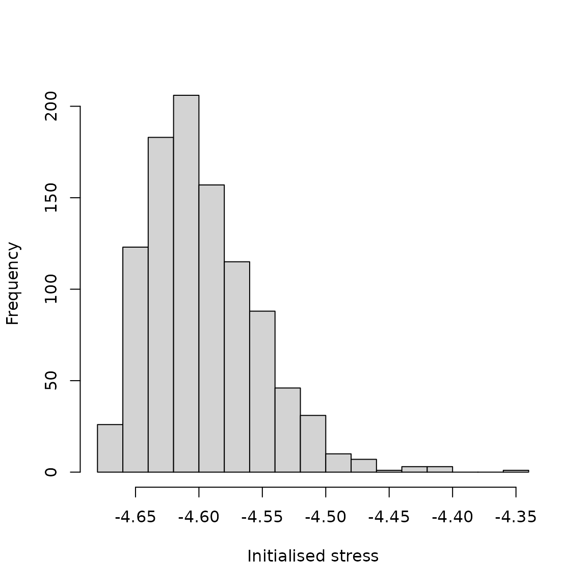
Figure 1. Distribution of stress for initialised
pest trait covariances in the resevol R package. Stress values are
computed using genome values produced by the mine_gmatrix
function for 1000 replicate populations of initialised pest loci
values.
If we are satisfied with the distribution of stress, then we can
accept mg as the genome for our initialised pests. The
whole contents of mg will then be passed on to the
run_farm_sim function, which initialises pests using the
genome values in mg before running simulations. Before
doing any of this, because we want to run a simulation on a customised
landscape, we will explain how such a landscape can be generated and
inserted into the simulation.
Landscape
Default settings for running simulations with the
run_farm_sim function create a spatially explicitly
landscape with dimensions specified by arguments xdim and
ydim, and a number of farms specified by
farms. These arguments can be over-ridden with a matrix
that defines landscape cell identities, which is set in the
terrain argument. A very simple custom 12 by 12 landscape
might look something like the below.
simple_terrain              <- matrix(data = 0, nrow = 12, ncol = 12)
simple_terrain[1:2, 1:3]    <- 1;
simple_terrain[3:7, 1:2]    <- 1;
simple_terrain[8:12, 1:2]   <- 2;
simple_terrain[1:2, 6:9]    <- 3;
simple_terrain[3:6, 7:9]    <- 3;
simple_terrain[1:6, 10:12]  <- 4;
simple_terrain[10:12, 7]    <- 5;
simple_terrain[7:12, 8:12]  <- 5;
simple_terrain[3:12, 3:4]   <- 6;
simple_terrain[7:9, 5]      <- 6;
simple_terrain[1:2, 4:5]    <- 7;
simple_terrain[3:6, 5:6]    <- 7;
simple_terrain[7:9, 6:7]    <- 7;
simple_terrain[10:12, 5:6]  <- 7;
print(simple_terrain)
## [,1] [,2] [,3] [,4] [,5] [,6] [,7] [,8] [,9] [,10] [,11] [,12]
## [1,] 1 1 1 7 7 3 3 3 3 4 4 4
## [2,] 1 1 1 7 7 3 3 3 3 4 4 4
## [3,] 1 1 6 6 7 7 3 3 3 4 4 4
## [4,] 1 1 6 6 7 7 3 3 3 4 4 4
## [5,] 1 1 6 6 7 7 3 3 3 4 4 4
## [6,] 1 1 6 6 7 7 3 3 3 4 4 4
## [7,] 1 1 6 6 6 7 7 5 5 5 5 5
## [8,] 2 2 6 6 6 7 7 5 5 5 5 5
## [9,] 2 2 6 6 6 7 7 5 5 5 5 5
## [10,] 2 2 6 6 7 7 5 5 5 5 5 5
## [11,] 2 2 6 6 7 7 5 5 5 5 5 5
## [12,] 2 2 6 6 7 7 5 5 5 5 5 5What is important is that the matrix elements only include natural numbers from 1 to the total number of farms (not skipping any numbers). In the case of the above, numbers 1-7 all appear on the landscape, so the matrix will work. We can visualise the matrix more clearly by looking at it as an image (Figure 2).

Figure 2. Image representing a simple landscape for the resevol package created from a 12 by 12 matrix of natural numbers from 1-7.
In Figure 2, each colour represents a unique farm, and colours
correspond to the numbers within the matrix simple_terrain
(note that the orientation differs between the matrix and the image).
This is a simple example, but matrices can be made large to model highly
complex landscapes. Additionally, not every colour needs to represent a
‘farm’ per se. We can represent other types of terrain such as
grassland, woodland, or water with its own natural number. The trick in
this case is to have each of these other types of terrain grow a crop
and use a pesticide that has no effect on pests (i.e., cannot be
consumed). If terrain types have no effect on pests, then they can
effectively model land that is not used for farming. We can show this
using the matrix land_eg, which is also included in the
resevol package. The dimensions of the landscape modelled in
land_eg are 128 by 128 cells, and the landscape includes 14
farms (1-14), grassland (15), forest (16), and water (17). The code
below produces an image that shows how these terrain types are
distributed over the landscape (Figure 3).
land_file <- system.file("landscape_eg.csv", package = "resevol");
land_dat  <- read.csv(file = land_file, header = FALSE);
land_eg   <- t(as.matrix(land_dat));
farm_cols <- c("#f4eadc", "#6a4b20", "#cea05f", "#e1c59d", "#a97833", "#cea05f",
               "#f2e6d6", "#6a4b20", "#cc9c59", "#dfc197", "#a27331", "#f0e3d0",
               "#5d421c", "#ca9852");
land_cols <- c(farm_cols, "#00ab41", "#234F1E", "#2832C2");
par(mar = c(0, 0, 0, 0));
image(land_eg, xaxt = "n", yaxt = "n", col = land_cols);
points(x = 0.2, y = 0.05, cex = 9, pch = 20);
text(x = 0.2, y = 0.05, labels = "1", cex = 2, col = "red");
points(x = 0.4, y = 0.1, cex = 9, pch = 20);
text(x = 0.4, y = 0.1, labels = "2", cex = 2, col = "red");
points(x = 0.4, y = 0.1, cex = 9, pch = 20);
text(x = 0.4, y = 0.1, labels = "2", cex = 2, col = "red");
points(x = 0.25, y = 0.27, cex = 9, pch = 20);
text(x = 0.25, y = 0.27, labels = "3", cex = 2, col = "red");
points(x = 0.20, y = 0.43, cex = 9, pch = 20);
text(x = 0.20, y = 0.43, labels = "4", cex = 2, col = "red");
points(x = 0.42, y = 0.48, cex = 9, pch = 20);
text(x = 0.42, y = 0.48, labels = "5", cex = 2, col = "red");
points(x = 0.28, y = 0.58, cex = 9, pch = 20);
text(x = 0.28, y = 0.58, labels = "6", cex = 2, col = "red");
points(x = 0.1, y = 0.8, cex = 9, pch = 20);
text(x = 0.1, y = 0.8, labels = "7", cex = 2, col = "red");
points(x = 0.7, y = 0.05, cex = 9, pch = 20);
text(x = 0.7, y = 0.05, labels = "8", cex = 2, col = "red");
points(x = 0.9, y = 0.2, cex = 9, pch = 20);
text(x = 0.9, y = 0.2, labels = "9", cex = 2, col = "red");
points(x = 0.85, y = 0.4, cex = 9, pch = 20);
text(x = 0.85, y = 0.4, labels = "10", cex = 2, col = "red");
points(x = 0.92, y = 0.58, cex = 9, pch = 20);
text(x = 0.92, y = 0.58, labels = "11", cex = 2, col = "red");
points(x = 0.88, y = 0.76, cex = 9, pch = 20);
text(x = 0.88, y = 0.76, labels = "12", cex = 2, col = "red");
points(x = 0.86, y = 0.93, cex = 9, pch = 20);
text(x = 0.86, y = 0.93, labels = "13", cex = 2, col = "red");
points(x = 0.52, y = 0.91, cex = 9, pch = 20);
text(x = 0.52, y = 0.91, labels = "14", cex = 2, col = "red");
points(x = 0.05, y = 0.59, cex = 7, pch = 20);
text(x = 0.05, y = 0.59, labels = "15", cex = 1.7, col = "white");
points(x = 0.46, y = 0.28, cex = 7, pch = 20);
text(x = 0.46, y = 0.28, labels = "16", cex = 1.7, col = "white");
points(x = 0.62, y = 0.36, cex = 7, pch = 20);
text(x = 0.62, y = 0.36, labels = "17", cex = 1.7, col = "white");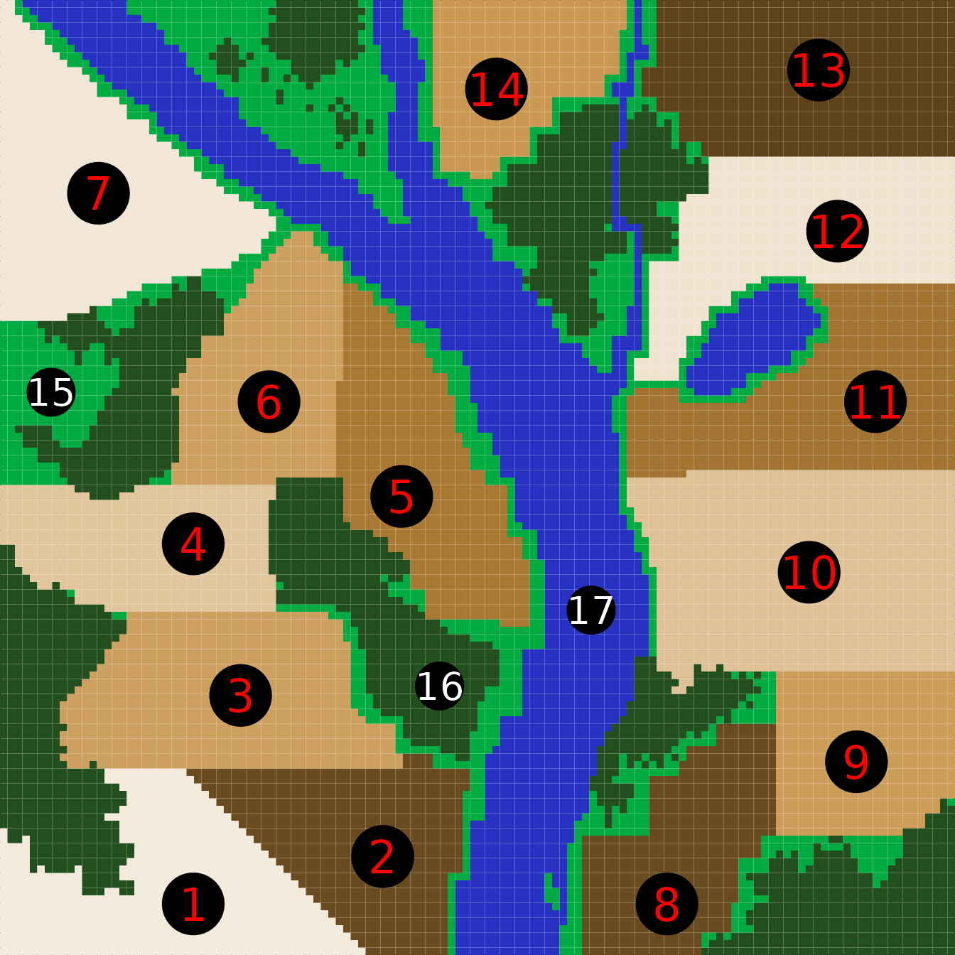
Figure 3. A complex landscape to be used in the resevol R package, including 14 separate farms, grassland, forest, and water. The image is represented in the code by a matrix in which element numbers correspond to different terrain colours (e.g., elements corresponding to water are numbered 17).
This land_eg matrix can be used in
run_farm_sim by setting terrain = land_eg. The
dimensions of the landscape will then automatically be set to
xdim = 128 and ydim = 128, and the number of
farms will be set to farms = 17. To ensure that we do not
have pests consuming crops or pesticides from non-farm areas, we just
need to set pest consumption options accordingly. Next, we describe how
this can be done by defining how crops and pesticides will be
initialised and rotated on the landscape.
Running simulations
We will simulate the same population twice using the mg
pest genome and land_eg landscape described
above under two different pesticide regimes, simulation 1 and
simulation 2. In both regimes, the same pesticide is applied to farms
that occupy the same side of the river (e.g., farms 1-7 apply pesticide
1 and farms 8-14 apply pesticide 2). In simulation 1, the pesticide is
never rotated. In simulation 2, farms rotate between pesticides 1 and 2
every 9 time steps. First, we will demonstrate how to customise crop and
pesticide rotation for simulation 1, then run the simulation, and
finally show the output. Second, we will repeat the process for
simulation 2 and demonstrate how comparisons can be made between the two
simulations.
Simulation 1
First, we focus on how to set custom pesticide
and crop rotation for simulations. Next, we run simulation 1 with the
run_farm_sim function. Finally, we demonstrate how to
interpret output for simulation 1.
Custom pesticide and crop rotation
The run_farm_sim arguments crop_init and
crop_rotation_type specify starting crops for each farm and
how crops rotate, respectively. Equivalent arguments
pesticide_init and pesticide_rotation_type
similarly specify starting pesticides and pesticide rotations,
respectively. We can set each argument to a number as a short-hand way
of specifying these parameters. For example, the default initialisation
crop_init = "random" simply causes each farm to start the
simulation with a random crop. Setting values of
crop_rotation_type to 1, 2, or 3 causes no rotation, random
rotation, or cycling through crop numbers in sequence, respectively. But
we can generate more specific initialisation and rotation types using a
vector to initialise crops and pesticides, and using a matrix to define
rotation. For initialisation, vector elements correspond to farm number
and element values correspond to the crop initialised. For our example
with 17 unique zones of terrain on the landscape, we can define
initialised crop choice as follows.
initial_crop <- c(1, 1, 1, 1, 1, 1, 1, 2, 2, 2, 2, 2, 2, 2, 3, 3, 3);That is, the first 7 farms on one side of the river all start off growing crop 1. Farms 8-14 all start off growing crop 2. Crop 3 is used as a dummy for grassland (15), forest (16), and water (17). We explain how to ensure that 15-17 is never used by pests below. Meanwhile, we can specify a matrix for the crop rotation regime. This regime will cause farmers to rotate between crops 1 and 2, but zones 15-17 to always use ‘crop’ 3.
rotate_crop       <- matrix(data = 0, nrow = 3, ncol = 3);
rotate_crop[1, 2] <- 1;
rotate_crop[2, 1] <- 1;
rotate_crop[3, 3] <- 1;
print(rotate_crop);
## [,1] [,2] [,3]
## [1,] 0 1 0
## [2,] 1 0 0
## [3,] 0 0 1In the above rotate_crop, matrix elements define the
probability of transitioning from one crop type (rows) to another crop
type (columns). Hence, in rotate_crop, farms that have been
applying crop 1 will always switch to crop 2, and vice versa. Landscape
zones applying crop 3 will never transition to any other crop, nor will
any other crop transition to type 3. We can set initial pesticides and
pesticide rotation in the same way. First we set initial pesticide
use.
initial_pesticide <- c(1, 1, 1, 1, 1, 1, 1, 2, 2, 2, 2, 2, 2, 2, 3, 3, 3);Next, we define pesticide rotation. Recall that in simulation 1, pesticides will not rotate and farms will maintain the same pesticide type over all time steps.
rotate_pesticide           <- matrix(data = 0, nrow = 3, ncol = 3);
rotate_pesticide[1, 1]     <- 1;
rotate_pesticide[2, 2]     <- 1;
rotate_pesticide[3, 3]     <- 1;
print(rotate_pesticide);
## [,1] [,2] [,3]
## [1,] 1 0 0
## [2,] 0 1 0
## [3,] 0 0 1We therefore have set farms to always use one of two crops and one of
two pesticides. Everything that is not a farm will use crop 3 and
pesticide 3. Next, we bring everything together and show how pests, the
landscape, and the rotation of crops and pesticides can be used in
run_farm_sim for simulations.
Running simulation 1
The code below runs simulation 1 using the run_farm_sim
function.
set.seed(2022);
sim1       <- run_farm_sim(mine_output             = mg,
                          terrain                  = land_eg,
                          crop_init                = initial_crop,
                          crop_rotation_type       = rotate_crop,
                          pesticide_init           = initial_pesticide,
                          pesticide_rotation_type  = rotate_pesticide,
                          food_consume             = c("T1", "T2", 0),
                          pesticide_consume        = c("T3", "T4", 0),
                          crop_number              = 3,
                          pesticide_number         = 3,
                          trait_means              = c(2, 2, 0.0, 0.0),
                          max_age                  = 6,
                          min_age_feed             = 0,
                          max_age_feed             = 2,
                          min_age_move             = 3,
                          max_age_move             = 6,
                          min_age_metabolism       = 3,
                          max_age_metabolism       = 6,
                          metabolism               = 0.5,
                          food_needed_surv         = 1,
                          reproduction_type        = "food_based",
                          food_needed_repr         = 2,
                          N                        = 1000,
                          repro                    = "biparental",
                          mating_distance          = 4,
                          rand_age                 = TRUE,
                          pesticide_tolerated_surv = 2,
                          movement_bouts           = 4,
                          move_distance            = 2,
                          crop_per_cell            = 10,
                          crop_sd                  = 0,
                          pesticide_per_cell       = 1,
                          pesticide_sd             = 0,
                          crop_rotation_time       = 18,
                          pesticide_rotation_time  = 9,
                          time_steps               = 240,
                          pesticide_start          = 81,
                          immigration_rate         = 100,
                          land_edge                = "reflect",
                          mutation_pr              = 0.01,
                          crossover_pr             = 0.01,
                          print_gens              = TRUE,
                          print_last              = TRUE);
Immediately below the first six arguments, we have the arguments
food_consume, pesticide_consume,
crop_number, and pesticide_number. The way
that these arguments are set ensures that pests only interact with farm
cells. The rate of food consumption for the first two crops is defined
by the values of traits 1 and 2 and set as "T1" and
"T2", respectively. The rate of consumption for crop 3 is
set to 0, meaning that no food can be eaten on these cells. Similarly,
the rate at which pesticides 1 and 2 are consumed is defined by the
values of traits 3 and 4, which are set as "T3" and
"T4", respectively. The rate of consumption for pesticide 3
is set to 0 so that pesticide is not consumed on these cells.
We next set the mean values of traits at the start of the simulation
with the argument trait_means. Mean consumption rate of
both crops is set to 2, while mean pesticide consumption rate is set to
0 (note, negative consumption rate values are possible, but are realised
as no consumption). Pests live up to 6 time steps
(max_age = 6), and are defined to start feeding upon birth
(min_age_feed = 0) and stop at age 2
(max_age_feed = 2). At age 3, pests start to move
(min_age_move = 3) and metabolise food
(min_age_metabolism = 3) at a rate of
metabolism = 0.5. The metabolism argument
defines the amount of consumed food lost during the time step, which can
affect pests when food consumed affects survival
(food_needed_surv) and reproduction
(reproduction_type). By setting
reproduction_type = "food_based" and
food_needed_surv = 1, we model a system in which pests burn
the food consumed from ages 0-2 at a rate of 0.5 units per time step
after age 3, then die when their reserves drop below 1. By setting
food_needed_repr = 2, we ensure that only pests that have 2
or more units of food stored can reproduce. Note that if we desired, we
could also set food_needed_surv,
food_needed_repr, and metabolism to be
evolving traits.
We initialise the population with N = 1000 obligately
biparental (repro = "biparental") pests, and can find a
mate within mating_distance = 4 cells of their own cell.
All pests are initialised at a random age
(rand_age = TRUE). Pests will die if they consume more than
2 total units of pesticide (pesticide_tolerated_surv = 2).
In each time step, pests that are able to move will do so an average of
4 times on the landscape (movement_bouts = 4), moving up to
2 cells in any direction during each bout
(movement_distance = 2). Recall that since pests consume
food and pesticide only between ages 0-2, then start moving at age 3, no
food or pesticide consumption occurs during movement (if applicable, it
could be turned on with feed_while_moving = TRUE and
pesticide_while_moving = TRUE). Each farm cell produces 10
units of crops (crop_per_cell = 10 and
crop_sd = 0) and 1 unit of pesticide
(pesticide_per_cell = 1 and pesticide_sd = 0).
Crops are rotated every 18 time steps
(crop_rotation_time = 18), and pesticides are set to rotate
every 9 time steps (pesticide_rotation_time = 9), but this
pesticide rotation has no effect in simulation 1 because the same
pesticide is applied upon rotation (as defined by
rotate_pesticide). This can be conceptualised as modelling
an 18 time step growing season in which pesticides are re-applied at the
start and halfway point of a season. Note that it is critical to
consider that crops are therefore refreshed every 18 time steps, not
every time step. Hence, any food consumed by a pest will be lost from a
cell and not replenished until crop rotation occurs. Because more than
one pest can occupy a single cell, crop loss can occur quickly depending
on how parameter values are set.
Lastly, we set the number of time steps to
time_steps = 240, and we set
pesticide_start = 81, which means that pesticides are not
applied at all until after a burn-in of 81 time steps. In each time
step, an average of 100 immigrants enter the population
(immigration_rate = 100). We set the landscape edge type to
land_edge = "reflect" to model a reflective edge in which
pests that attempt to leave one side of the landscape bounce back toward
the centre. Pest genome mutation rate and crossover rate at a locus are
set to mutation_pr = 0.01 and
crossover_pr = 0.01, respectively. We print out the
dynamics of the evolving population over time, and all of the individual
data from the last time step, to two separate CSV files (individual data
are not included in the package due to its size). All arguments of
run_farm_sim not mentioned are set to default parameter
values, which can be found in the package documentation.
Simulation 1 output
When running the function run_farm_sim, the population
size of the pest will be printed in the R console in each time step.
This is primarily because simulations can take a long time, and printing
makes it possible to estimate how much time is remaining. Printing to
the console can be turned off by setting
print_gens = FALSE. Once the simulation has finished, two
CSV files will be created in the working directory. The file
“population_data.csv” saves population data over time, and
“individuals.csv” saves every characteristic of all individuals in the
last time step (including full individual genomes). Here we show how to
work with the most relevant information from these two files to make
inferences about pest population and evolutionary dynamics.
We will start with the population level output that is printed to “population_data.csv”, which has been renamed “population_data_sim1.csv”.
population_data_file_sim1 <- system.file("population_data_sim1.csv",
                                         package = "resevol");
population_data_sim1      <- read.csv(file = population_data_file_sim1);
This file includes population-level parameters of population size and
mean pest age, sex, food consumed, pesticide consumed, mortality rate,
and trait values reported for each time step. If
get_f_coef = TRUE in run_farm_sim, then mean
inbreeding coefficients of pests are also reported.
##   time_step population_size mean_age mean_sex mean_food_consumed
## 1         0            1000 3.982000 2.499000           0.396658
## 2         1             301 1.813953 2.498339           2.590001
## 3         2             415 2.166265 2.474699           2.708252
## 4         3             540 2.412963 2.488889           2.830218
## 5         4             756 2.488095 2.469577           2.755487
## 6         5             964 2.452282 2.484440           2.819527
##   mean_pesticide_consumed mortality_rate mean_food1_consumed
## 1                       0       0.837000            0.179506
## 2                       0       0.205980            0.578690
## 3                       0       0.233735            0.417990
## 4                       0       0.218519            0.398647
## 5                       0       0.279101            0.411980
## 6                       0       0.312241            0.405805
##   mean_food2_consumed mean_food3_consumed mean_pesticide1_consumed
## 1            0.217152                   0                        0
## 2            0.738026                   0                        0
## 3            0.526348                   0                        0
## 4            0.521056                   0                        0
## 5            0.496357                   0                        0
## 6            0.468015                   0                        0
##   mean_pesticide2_consumed mean_pesticide3_consumed trait1_mean_value
## 1                        0                        0          1.998091
## 2                        0                        0          1.962117
## 3                        0                        0          2.021925
## 4                        0                        0          2.020423
## 5                        0                        0          2.073448
## 6                        0                        0          2.083852
##   trait2_mean_value trait3_mean_value trait4_mean_value mean_f
## 1          2.014113          0.001834          0.003205      0
## 2          2.140079          0.041814          0.000534      0
## 3          2.211915          0.067218          0.029188      0
## 4          2.279216          0.034372          0.089154      0
## 5          2.313421          0.099480          0.059904      0
## 6          2.367128          0.105447          0.080354      0
Because the structure of the data frame above depends on the number of crops, pesticides, and evolving traits simulated, there are no pre-set functions in the resevol package for plotting. Here we include code for plotting population size, consumption of the two food types, two pesticides types, and evolving trait means. Note that because crop and pesticide 3 are dummy variables (not consumed at all), we do not need to plot these. Figure 4 shows how population density of pests changes over time.
mbox <- function(x0, x1, y0, y1){
    xx <- seq(from=x0, to=x1, length.out = 100);
    yy <- seq(from=y0, to=y1, length.out = 100);
    xd <- c(rep(x0, 100), xx, rep(x1,100), rev(xx));
    yd <- c(yy, rep(y1,100), rev(yy), rep(y0, 100));
    return(list(x=xd, y=yd));
}
season          <- seq(from = 0, to = 240, by = 18);
blocks          <- length(season) - 1;
plot(x = population_data_sim1[["time_step"]], type = "n",
     y = population_data_sim1[["population_size"]], cex.lab = 1.25,
     cex.axis = 1.25, ylab = "Pest population abundance", xlab = "Time step",
     ylim = c(0, max(population_data_sim1[["population_size"]])));
for(i in 1:blocks){
    rbox <- mbox(x0 = season[i], x1 = season[i + 1], y0 = -1000, y1 = 21000);
    if(i %% 2 == 0){
        polygon(x = rbox$x, y = rbox$y, lwd = 3, border = NA,
                col = "grey90");
    }
}
points(x = population_data_sim1[["time_step"]],
     y = population_data_sim1[["population_size"]], type = "l", lwd = 2);
abline(v = 81, lwd = 3, col = "red");
box();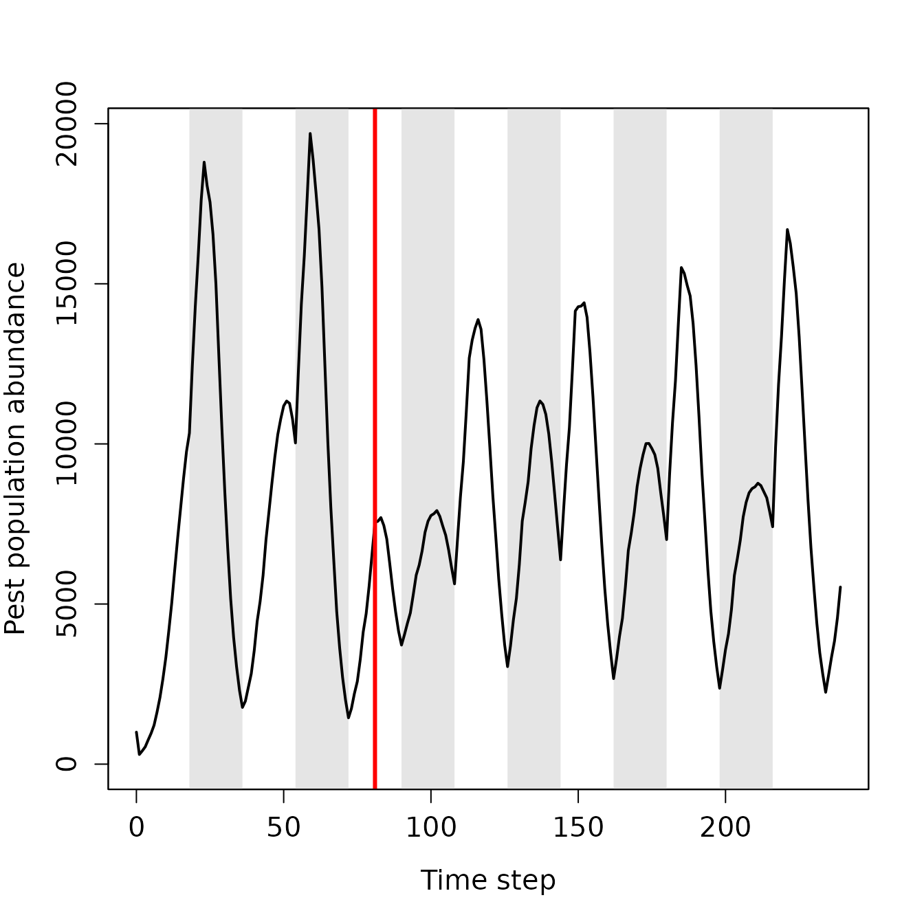
Figure 4. Pest abundance over time in a population simulated using the resevol R package in which pesticides are not rotated over time. The grey shaded regions show individual crop seasons; pesticides are applied at the start and midpoint of each seasons, beginning at the time step indicated by the red vertical line.
Figure 5 shows how the mean consumption of different foods and pesticides changes over time.
par(mfrow = c(2, 2), mar = c(1, 4, 1, 1));
plot(x = population_data_sim1[["time_step"]], type = "n", ylim = c(0, 0.8),
     y = population_data_sim1[["mean_food1_consumed"]], cex.lab = 1.25,
     ylab = "Mean crop 1 consumed", xlab = "Time step", xaxt = "n");
for(i in 1:blocks){
    rbox <- mbox(x0 = season[i], x1 = season[i + 1], y0 = -1000, y1 = 6000);
    if(i %% 2 == 0){
        polygon(x = rbox$x, y = rbox$y, lwd = 3, border = NA,
                col = "grey90");
    }
}
points(x = population_data_sim1[["time_step"]],
       y = population_data_sim1[["mean_food1_consumed"]], type = "l", lwd = 2);
text(x = 5, y = 0.79, labels = "a", cex = 2);
box();
par(mar = c(1, 4, 1, 1));
plot(x = population_data_sim1[["time_step"]], type = "n", ylim = c(0, 0.8),
     y = population_data_sim1[["mean_food2_consumed"]], cex.lab = 1.25 ,
     ylab = "Mean crop 2 consumed", xlab = "Time step", xaxt = "n");
for(i in 1:blocks){
    rbox <- mbox(x0 = season[i], x1 = season[i + 1], y0 = -1000, y1 = 6000);
    if(i %% 2 == 0){
        polygon(x = rbox$x, y = rbox$y, lwd = 3, border = NA,
                col = "grey90");
    }
}
points(x = population_data_sim1[["time_step"]],
       y = population_data_sim1[["mean_food2_consumed"]], type = "l", lwd = 2);
text(x = 5, y = 0.79, labels = "b", cex = 2);
box();
par(mar = c(4, 4, 1, 1));
plot(x = population_data_sim1[["time_step"]], type = "n", ylim = c(0, 0.8),
     y = population_data_sim1[["mean_pesticide1_consumed"]], cex.lab = 1.25,
     ylab = "Mean pesticide 1 consumed", xlab = "Time step");
for(i in 1:blocks){
    rbox <- mbox(x0 = season[i], x1 = season[i + 1], y0 = -1000, y1 = 6000);
    if(i %% 2 == 0){
        polygon(x = rbox$x, y = rbox$y, lwd = 3, border = NA,
                col = "grey90");
    }
}
points(x = population_data_sim1[["time_step"]],
       y = population_data_sim1[["mean_pesticide1_consumed"]], type = "l", lwd = 2);
box();
text(x = 5, y = 0.78, labels = "c", cex = 2);
par(mar = c(4, 4, 1, 1));
plot(x = population_data_sim1[["time_step"]], type = "n", ylim = c(0, 0.8),
     y = population_data_sim1[["mean_pesticide2_consumed"]], cex.lab = 1.25,
     ylab = "Mean pesticide 2 consumed", xlab = "Time step");
for(i in 1:blocks){
    rbox <- mbox(x0 = season[i], x1 = season[i + 1], y0 = -1000, y1 = 6000);
    if(i %% 2 == 0){
        polygon(x = rbox$x, y = rbox$y, lwd = 3, border = NA,
                col = "grey90");
    }
}
points(x = population_data_sim1[["time_step"]],
       y = population_data_sim1[["mean_pesticide2_consumed"]], type = "l",
       lwd = 2);
box();
text(x = 5, y = 0.78, labels = "d", cex = 2);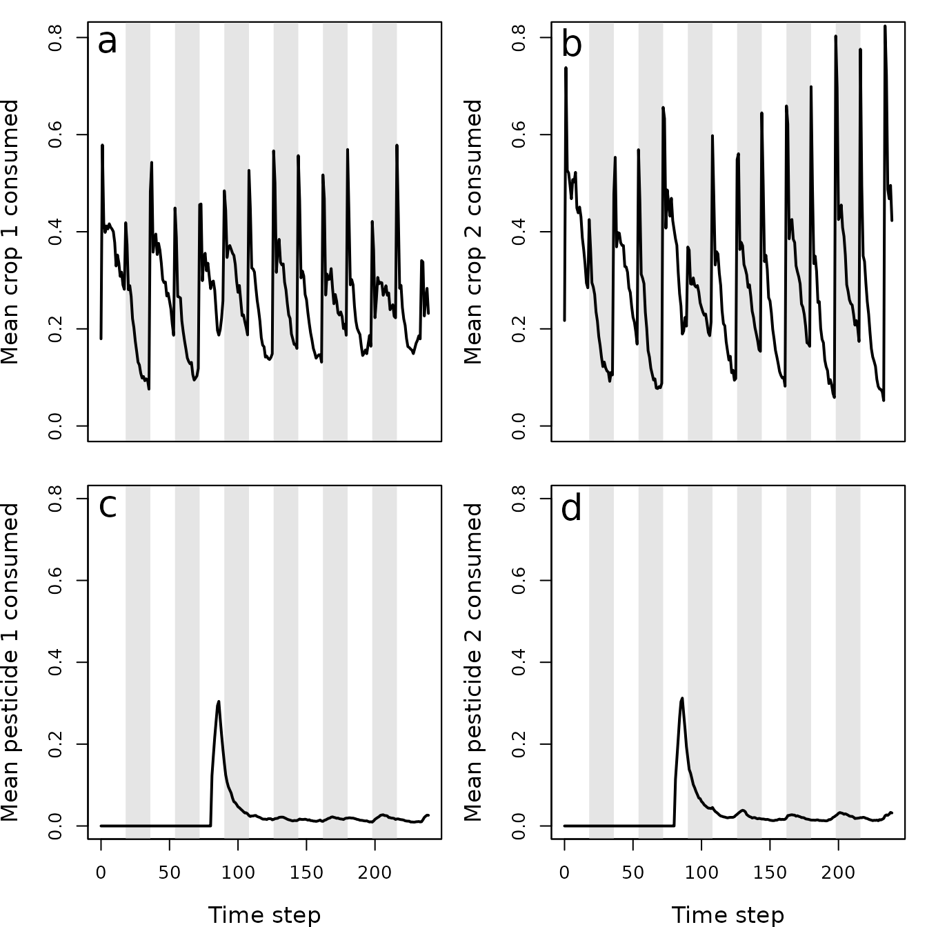
Figure 5. Pest consumption over time in a population simulated using the resevol R package in which pesticides are not rotated over time. Panels show (a) mean amount of crop 1 and (b) crop 2 consumed per pest, and (c) mean amount of pesticide 1 and (d) pesticide 2 consumed per pest. Grey shaded regions show individual crop seasons; pesticides are applied at the start and midpoint of each seasons, beginning at the time step 100.
Similarly, we can visualise how all four traits evolve over time (Figure 6).
par(mfrow = c(2, 2), mar = c(1, 4, 1, 1));
plot(x = population_data_sim1[["time_step"]], type = "n", ylim = c(2, 3.6),
     y = population_data_sim1[["trait1_mean_value"]], cex.lab = 1.25,
     ylab = "Mean crop 1 consumption trait", xlab = "Time step", xaxt = "n");
for(i in 1:blocks){
    rbox <- mbox(x0 = season[i], x1 = season[i + 1], y0 = -1000, y1 = 6000);
    if(i %% 2 == 0){
        polygon(x = rbox$x, y = rbox$y, lwd = 3, border = NA,
                col = "grey90");
    }
}
points(x = population_data_sim1[["time_step"]],
     y = population_data_sim1[["trait1_mean_value"]], type = "l", lwd = 2);
text(x = 5, y = 3.56, labels = "a", cex = 2);
box();
par(mar = c(1, 4, 1, 1));
plot(x = population_data_sim1[["time_step"]], type = "n", ylim = c(2, 3.6),
     y = population_data_sim1[["trait2_mean_value"]], cex.lab = 1.25 ,
     ylab = "Mean crop 2 consumption trait", xlab = "Time step", xaxt = "n");
for(i in 1:blocks){
    rbox <- mbox(x0 = season[i], x1 = season[i + 1], y0 = -1000, y1 = 6000);
    if(i %% 2 == 0){
        polygon(x = rbox$x, y = rbox$y, lwd = 3, border = NA,
                col = "grey90");
    }
}
points(x = population_data_sim1[["time_step"]],
       y = population_data_sim1[["trait2_mean_value"]], type = "l", lwd = 2);
text(x = 5, y = 3.56, labels = "b", cex = 2);
box();
par(mar = c(4, 4, 1, 1));
plot(x = population_data_sim1[["time_step"]], type = "n", ylim = c(-0.8, 1.4),
     y = population_data_sim1[["trait3_mean_value"]], cex.lab = 1.25,
     ylab = "Mean pesticide 1 consumption trait", xlab = "Time step");
for(i in 1:blocks){
    rbox <- mbox(x0 = season[i], x1 = season[i + 1], y0 = -1000, y1 = 6000);
    if(i %% 2 == 0){
        polygon(x = rbox$x, y = rbox$y, lwd = 3, border = NA,
                col = "grey90");
    }
}
points(x = population_data_sim1[["time_step"]],
       y = population_data_sim1[["trait3_mean_value"]], type = "l", lwd = 2);
box();
text(x = 5, y = 1.34, labels = "c", cex = 2);
par(mar = c(4, 4, 1, 1));
plot(x = population_data_sim1[["time_step"]], type = "n", ylim = c(-0.8, 1.4),
     y = population_data_sim1[["trait4_mean_value"]], cex.lab = 1.25,
     ylab = "Mean pesticide 2 consumption trait", xlab = "Time step");
for(i in 1:blocks){
    rbox <- mbox(x0 = season[i], x1 = season[i + 1], y0 = -1000, y1 = 6000);
    if(i %% 2 == 0){
        polygon(x = rbox$x, y = rbox$y, lwd = 3, border = NA,
                col = "grey90");
    }
}
points(x = population_data_sim1[["time_step"]],
       y = population_data_sim1[["trait4_mean_value"]], type = "l", lwd = 2);
box();
text(x = 5, y = 1.34, labels = "d", cex = 2);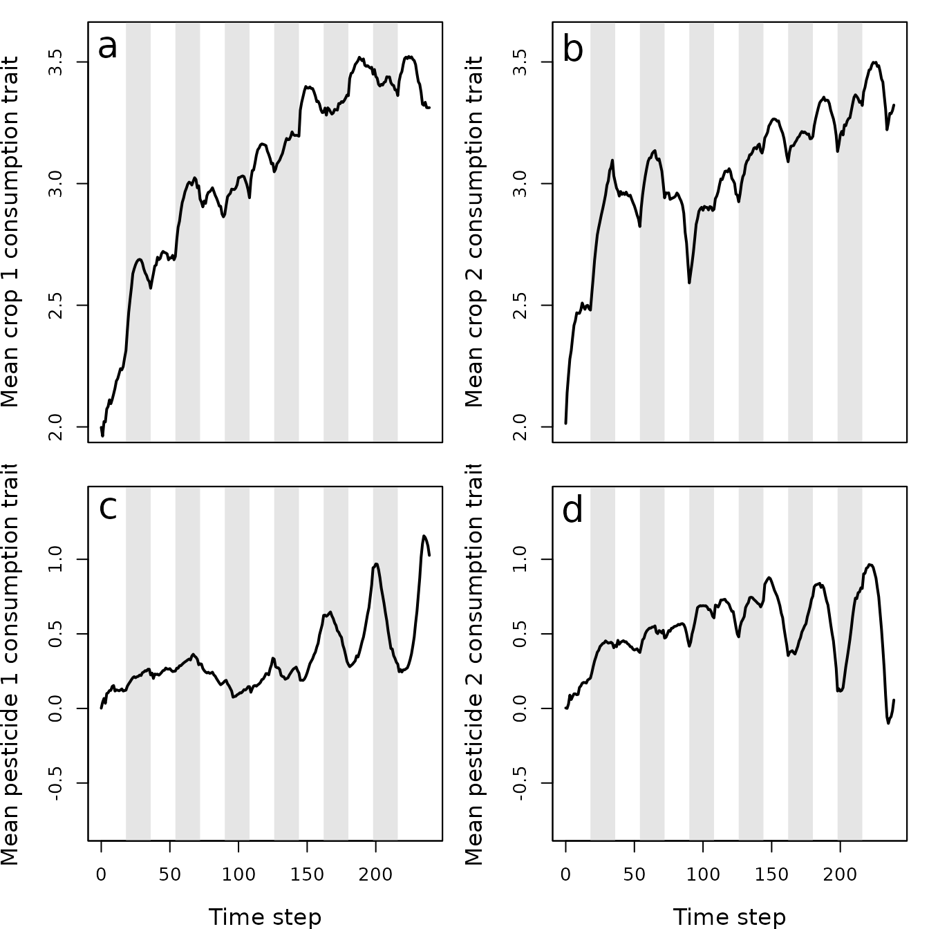
Figure 6. Mean values of pest traits T1 (crop 1 consumption rate), T2 (crop 2 consumption rate), T3 (pesticide 1 consumption rate), and T4 (pesticide 2 consumption rate) in a population simulated using the resevol R package in which pesticides are not rotated over time. Grey shaded regions show individual crop seasons; pesticides are applied at the start and midpoint of each seasons, beginning at the time step 100.
Next, we look at the file that includes the complete information for all individuals in the last time step of the simulation. Using this data set, we can examine the distribution of pests on the landscape, and the realised covariance of evolving pest traits. In this output “last_time_step.csv”, traits always begin in column 102, meaning that individual trait values for traits 1, 2, 3, and 4 will be in columns 102, 103, 104, and 105, respectively. In this example, the CSV output file “last_time_step.csv” has been renamed “last_time_step_sim1.csv”. To minimise the size of the resevol R package, all data columns except pest locations and traits have been removed from example outputs, so pest locations are in columns 1-2 (not 3-4) and traits are in columns 3-6 (not 102-105). The last time step output is read into R below.
last_time_step_file_sim1 <- system.file("last_time_step_sim1.csv",
                                        package = "resevol");
pop_last_time_step_sim1  <- read.csv(file = last_time_step_file_sim1);
We can plot the distribution over the landscape using the code below.
The code identifies the x-locations and y-locations of each pest
i in pop_last_time_step_sim1, and these
landscape cells are replaced with the number 18. A new land colour for
black #000000 is then included, and the map is reproduced
as an image in R. Figure 7 shows the same map as above, but with the
numbering removed to make the pests (black points) more visible.
par(mar = c(0, 0, 0, 0));
landscape    <- land_eg;
for(i in 1:dim(pop_last_time_step_sim1)[1]){
    xloc <- pop_last_time_step_sim1[i, 1] + 1;
    yloc <- pop_last_time_step_sim1[i, 2] + 1;
    landscape[xloc, yloc] <- 18;
}
land_cols <- c(land_cols, "#000000");
image(landscape, xaxt = "n", yaxt = "n", col = land_cols);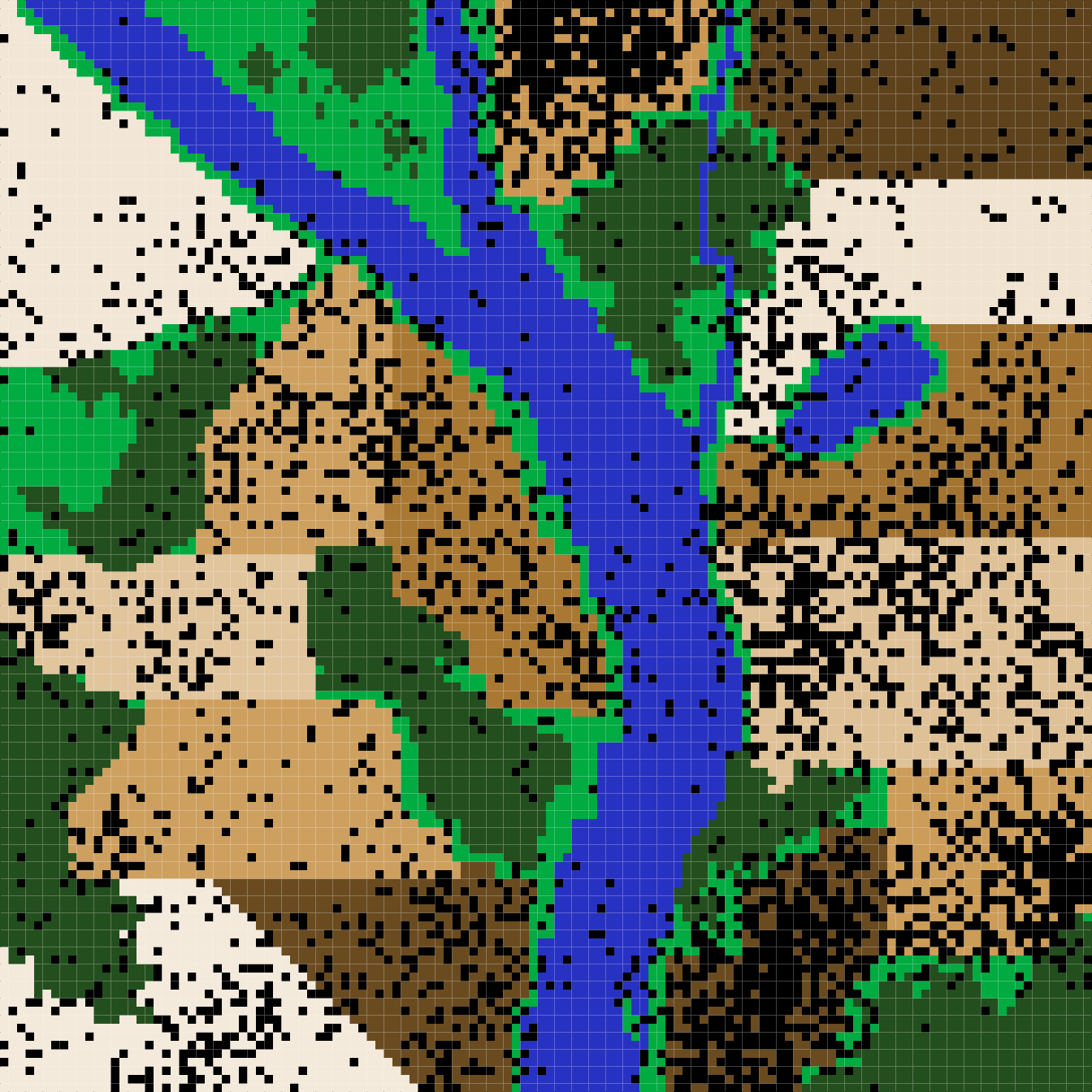
Figure 7. A complex landscape for simulating the ecology of pests and the evolution of pesticide resistance on farmland in the resevol R package. Terrain includes farms (brown colours), grassland (light green), forest (dark green), and water (blue). Black points show the locations of individual pests after 240 time steps for a simulation in which pesticides are not rotated over time.
head(pop_last_time_step_sim1);## V3 V4 V102 V103 V104 V105
## 1 33 13 2.395557 3.485652 -1.413820 2.185108
## 2 94 109 4.325184 1.408115 1.212488 -0.505254
## 3 108 58 4.583821 3.336972 2.907757 -1.297925
## 4 108 61 3.385105 2.619580 1.399597 -0.577378
## 5 2 47 3.713334 3.623724 -0.853502 2.222031
## 6 87 63 4.034968 3.601765 1.555337 -0.060638
print(land_cols);## [1] "#f4eadc" "#6a4b20" "#cea05f" "#e1c59d" "#a97833" "#cea05f" "#f2e6d6"
## [8] "#6a4b20" "#cc9c59" "#dfc197" "#a27331" "#f0e3d0" "#5d421c" "#ca9852"
## [15] "#00ab41" "#234F1E" "#2832C2" "#000000"The spatial pattern of pests over the landscape can be useful for visualising pest population dynamics. In the case of the above, pest density is higher on some farms (e.g., 1, 8, 9, 10, and 15) than others (e.g., 3, 12, and 13), and this pest density could be interpreted with respect to individual farm crop and pesticide rotation regimes. Hence, for the four evolving traits, a covariance matrix of pest traits can be calculated at the end of the simulation.
##            V102       V103       V104       V105
## V102  1.1223660 -0.1485266  0.2470207  0.1506317
## V103 -0.1485266  1.3351424 -0.0714354  0.5612672
## V104  0.2470207 -0.0714354  2.9213039 -2.8459986
## V105  0.1506317  0.5612672 -2.8459986  3.1352726
The above covariance matrix shows that after 240 time steps, the covariance between consumption of pesticides 1 and 2 has decreased from -0.3992066 to -2.8459986, suggesting that the trade-off for resisting pesticides had become stronger. In contrast, the covariance between consumption of crops 1 and 2 has increased from -0.4510309 to -0.1485266, suggesting that the trade-off in ability to consume crops of each type has weakened.
Simulation 2
We now repeat the simulations such that pesticide application is
rotated every 9 time steps. To make this rotation, we only need to
redefine rotate_pesticide.
rotate_pesticide           <- matrix(data = 0, nrow = 3, ncol = 3);
rotate_pesticide[1, 2]     <- 1;
rotate_pesticide[2, 1]     <- 1;
rotate_pesticide[3, 3]     <- 1;
Now, every 9 time steps, crops using pesticide 1 will switch to
pesticide 2, and crops using pesticide 2 will switch to pesticide 1. We
can re-run the same simulation with the same genome (mg),
landscape (land_eg), and simulation seed
(2022) used in simulation 1. Hence, the only thing changing
between the two simulations is the pesticide rotation.
set.seed(2022);
sim2       <- run_farm_sim(mine_output             = mg,
                          terrain                  = land_eg,
                          crop_init                = initial_crop,
                          crop_rotation_type       = rotate_crop,
                          pesticide_init           = initial_pesticide,
                          pesticide_rotation_type  = rotate_pesticide,
                          food_consume             = c("T1", "T2", 0),
                          pesticide_consume        = c("T3", "T4", 0),
                          crop_number              = 3,
                          pesticide_number         = 3,
                          trait_means              = c(2, 2, 0.0, 0.0),
                          max_age                  = 6,
                          min_age_feed             = 0,
                          max_age_feed             = 2,
                          min_age_move             = 3,
                          max_age_move             = 6,
                          min_age_metabolism       = 3,
                          max_age_metabolism       = 6,
                          metabolism               = 0.5,
                          food_needed_surv         = 1,
                          reproduction_type        = "food_based",
                          food_needed_repr         = 2,
                          N                        = 1000,
                          repro                    = "biparental",
                          mating_distance          = 4,
                          rand_age                 = TRUE,
                          pesticide_tolerated_surv = 2,
                          movement_bouts           = 4,
                          move_distance            = 2,
                          crop_per_cell            = 10,
                          crop_sd                  = 0,
                          pesticide_per_cell       = 1,
                          pesticide_sd             = 0,
                          crop_rotation_time       = 18,
                          pesticide_rotation_time  = 9,
                          time_steps               = 240,
                          pesticide_start          = 81,
                          immigration_rate         = 100,
                          land_edge                = "reflect",
                          mutation_pr              = 0.01,
                          crossover_pr             = 0.01,
                          print_gens              = TRUE,
                          print_last              = TRUE);
We can look at the same outputs for simulation 2 that we did for simulation 1. We first read in the output for simulation 2.
population_data_file_sim2 <- system.file("population_data_sim2.csv",
                                    package = "resevol");
population_data_sim2      <- read.csv(file = population_data_file_sim2);
To avoid needless repetition, the code for plots will not be included for simulation 2. Figure 8 shows population abundance over time for simulation 2.
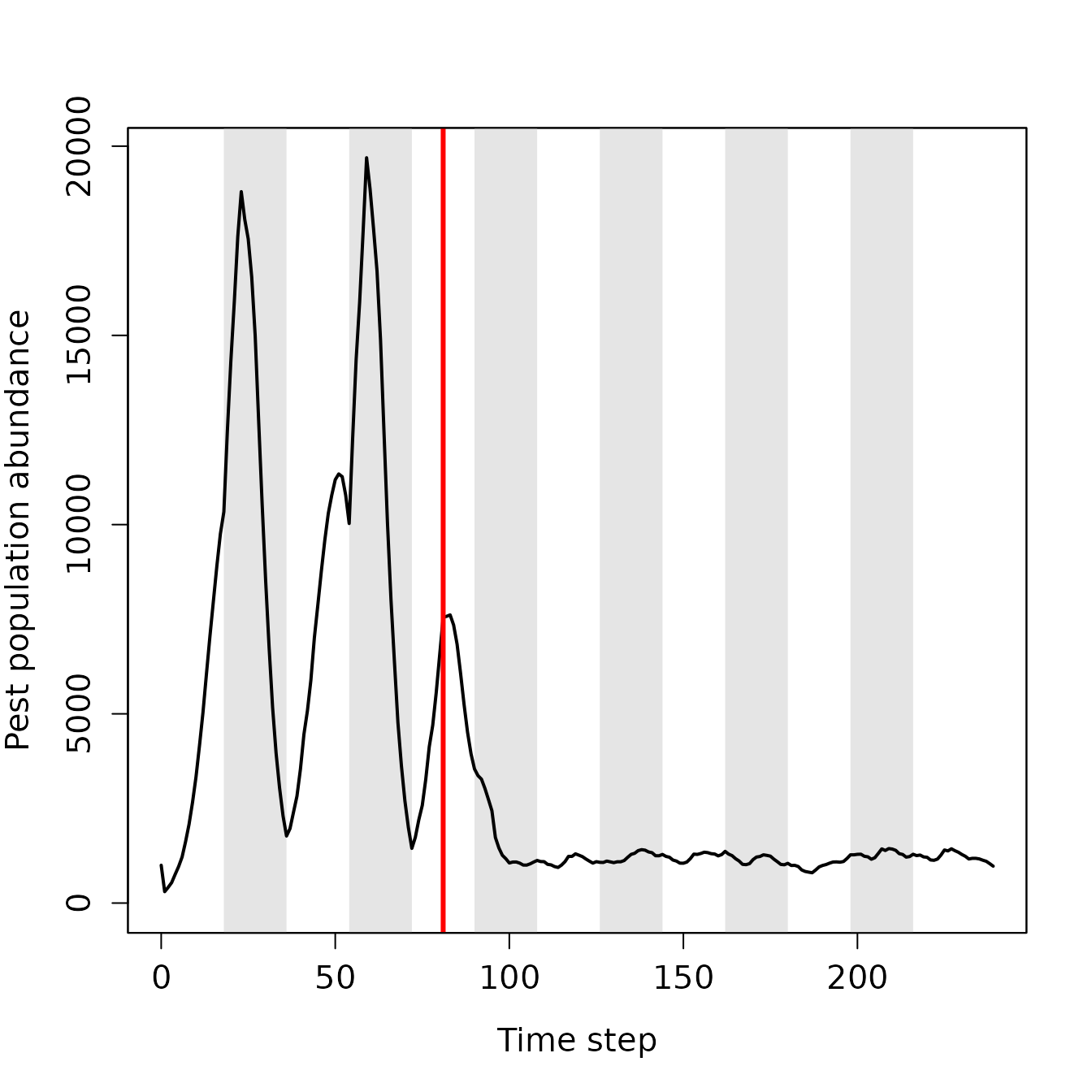
Figure 8. Pest abundance over time in a population simulated using the resevol R package in which pesticides rotates every 9 time steps. The grey shaded regions show individual crop seasons; pesticides are applied at the start and midpoint of each seasons, beginning at the time step indicated by the red vertical line.
After pesticides are applied at time step 81, pest population size decreases and does not recover. Figure 9 shows crop and pesticide consumption over time.
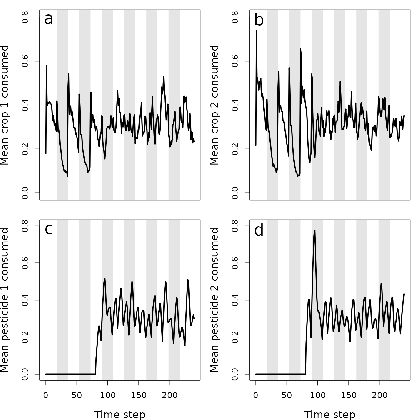
Figure 9. Pest consumption over time in a population simulated using the resevol R package in which pesticides rotate every 9 time steps. Panels show (a) mean amount of crop 1 and (b) crop 2 consumed per pest, and (c) mean amount of pesticide 1 and (d) pesticide 2 consumed per pest. Grey shaded regions show individual crop seasons; pesticides are applied at the start and midpoint of each seasons, beginning at the time step 100.
Figure 10 shows how pest traits evolve over time when pesticides are rotated.
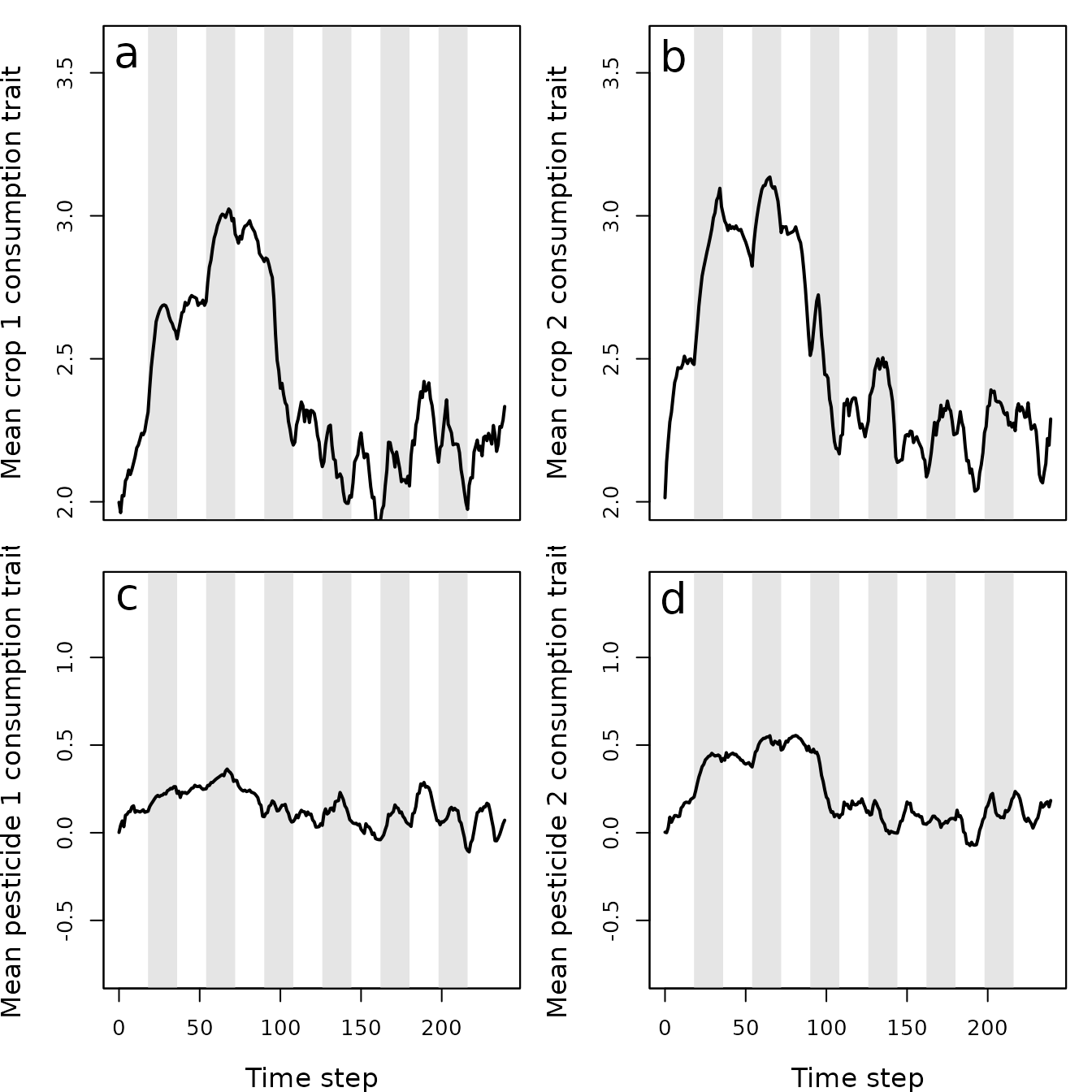
Figure 10. Mean values of pest traits T1 (crop 1 consumption rate), T2 (crop 2 consumption rate), T3 (pesticide 1 consumption rate), and T4 (pesticide 2 consumption rate) in a population simulated using the resevol R package in which pesticides rotate every 9 time steps. Grey shaded regions show individual crop seasons; pesticides are applied at the start and midpoint of each seasons, beginning at the time step 100.
We can observe the spatial distribution of pests on the landscape in the final time step (Figure 11).
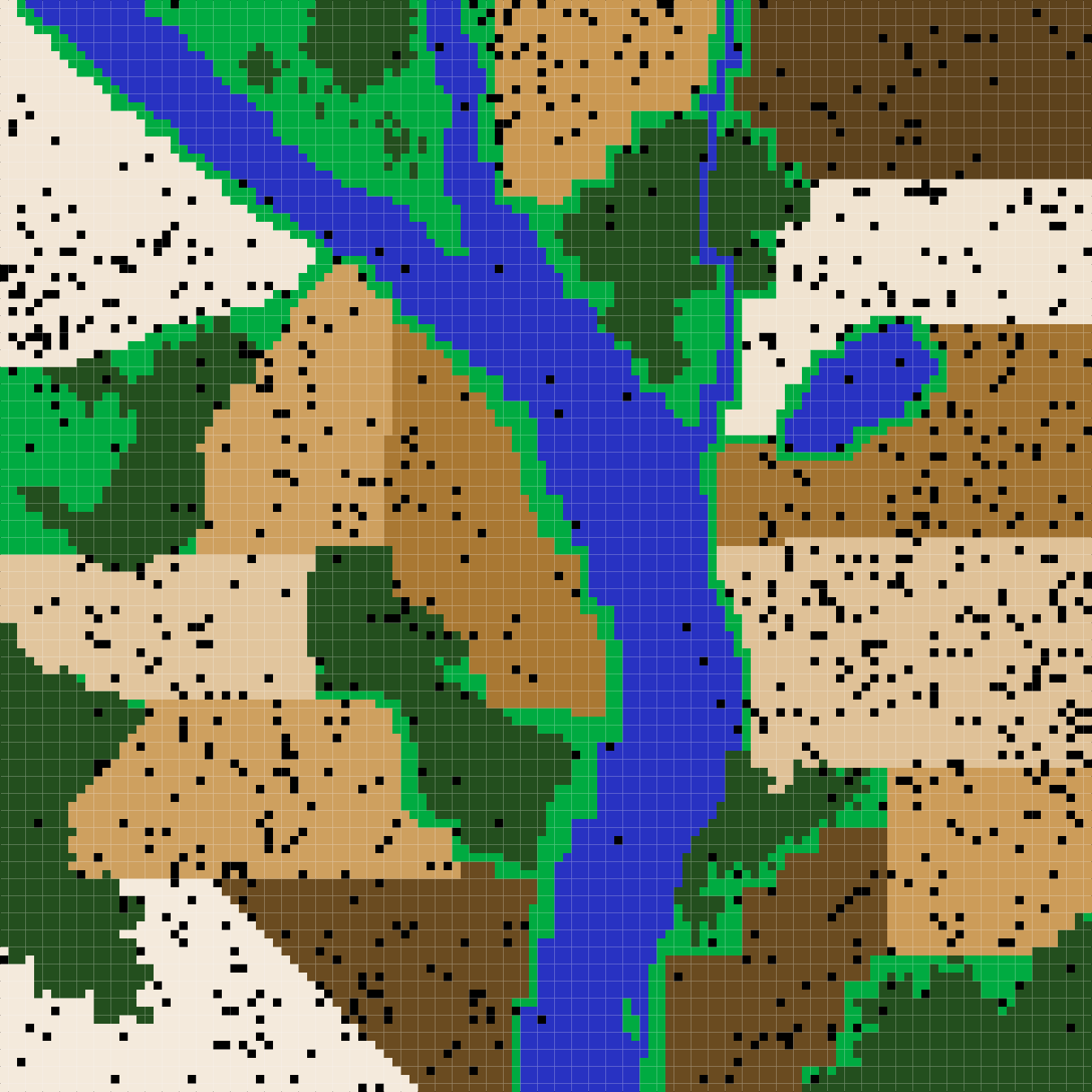
Figure 11. A complex landscape for simulating the ecology of pests and the evolution of pesticide resistance on farmland in the resevol R package. Terrain includes farms (brown colours), grassland (light green), forest (dark green), and water (blue). Black points show the locations of individual pests after 240 time steps for a simulation in which pesticides are not rotated over time.
Finally, we can examine the trait covariances in the final time step below.
##            V102        V103       V104        V105
## V102  1.5769217 -0.53211838  0.0665547  0.35835679
## V103 -0.5321184  1.29401550  0.2987174  0.01794992
## V104  0.0665547  0.29871744  0.9629416 -0.81135108
## V105  0.3583568  0.01794992 -0.8113511  0.96416686
We can use the outputs above to contrast the population dynamics of pests under a regime that lacks (simulation 1) or does not lack (simulation 2) the rotation of pesticide types.
Conclusion
From the output above, we can conclude that when farms rotate the pesticide that they apply between pesticide 1 and pesticide 2, it has a substantial effect on pest density and evolution. In the absence of pesticide rotation, the pest population quickly recovers after pesticides are first applied (Figure 4). Consequently, pesticides have very little long-term effect on the amount of crops consumed (Figure 5a,b), and while there is an initial spike in the consumption of both pesticides (Figure 5c,d), this consumption quickly declines. Despite the positive covariance between crop consumption and pesticide consumption, and the negative covariances between consumption of crop and pesticide types, these trade-offs appear to have only a modest effect on reducing actual crop consumption and maintaining or increasing pesticide consumption (Figure 6). Consequently, some farms experience high densities of pests that are resistant to the applied pesticides (Figure 7).
In contrast, when pesticides are rotated every 9 time steps, the pest population density drops after the onset of pesticide application and does not recover (Figure 8). The amount of each crop consumed per pests also drops (Figure 9a, b), while the amount of pesticide 1 and 2 consumed is maintained at a much higher rate than occurred in the absence of pesticide rotation (Figure 9c, d). Because selection against pesticide consumption was not consistent for a specific farm, and there is a trade-off between pest consumption of pesticide 1 versus 2, local adaptation to a single pesticide did not occur (Figure 10). Overall, farms therefore did not experience high densities of pests, and pest resistance to pesticide is well-managed (Figure 11).
Trait covariance differences between simulations 1 and 2 also highlight the effect that pesticide rotation had on pesticide resistance evolution. When no pesticide rotation occurred, the trade-off between consumption rate of pesticides 1 and 2 was reflected in a realised trait covariance of -2.8459986. But when pesticides were rotated, the realised covariance was instead -0.8113511. This means that in simulation 1, pests that are highly resistant to pesticide 1 were not highly resistant to pesticide 2, and vice versa. In other words, the lack of pesticide rotation resulted in local adaptation, with some pests specialising on resistance to one of the two pesticides. In simulation 2, pests maintained at least some resistance to both pesticides. Local adaptation was not possible because different pesticides were applied in sequence on any given farm.
This advanced example was not rigorous, but it illustrates how a
rigorous simulation of pesticide resistance evolution could be designed
with the resevol R package. To make robust predictions, multiple
replicate simulations would need to be run for the same set of
simulation conditions (in this case, for simulation 1 and 2) to account
for stochastic effects in the model. For example, we might repeat the
above initalisation of pest genomes to obtain 20
genomes with similar covariance structures, then run simulation 1 and simulation 2 20
times to get more robust predictions about pest population dynamics. We
might also need to consider a range of parameter values if some values
are unknown or uncertain (e.g., pest movement or trait means). To
develop theory, we could also contrast simulations with more fundamental
differences. For example, we might test how mating system affects
pesticide resistance evolution by running the same set of simulations
for repro = "asexual", repro = "sexual", and
repro = "biparental". The resevol R package is therefore a
highly flexible and powerful tool for running complex models tailored to
specific systems, and for developing theory on pest ecology, evolution,
and management.